
[Training a 500B LLM from Scratch] 19/25: Training Stopped. How Do We Pick Up Where We Left Off?
On day ten of training, at 10:40 a.m., a server went offline. The other machines soon stalled while waiting for communication. All 5,120 GPUs, advancing together a moment earlier, had stopped.
I opened the save log. The 10 a.m. checkpoint had completed.
That meant repeating the last 40 minutes of computation. The previous nine days still had a way back. The next steps were concrete: confirm that the checkpoint was usable, replace the failed machine, and continue through the data in its original order.
The storage capacity reserved in Part 13 had become the key to resuming training. I traced the interruption backward, starting with exactly what the 10 a.m. checkpoint contained.
First, What Does “Training Progress” Include?
The weight files tell us what the model has learned so far. Continuing training also requires knowing how it reached that point and what it was about to read next.
AdamW keeps a history of recent gradients. The learning-rate scheduler records whether training is in warmup or decay. The sampling program tracks the order and position of the material. Random states affect certain training operations. Together, these let us continue along the original training path.
We therefore save after a complete parameter update. At that point, all the shards have finished the same step, and gradient accumulation for the next step has not begun. Resuming with the next complete update gives the states a clear relationship.
| Saved content | What it tells us during recovery |
|---|---|
| Model weights and high-precision master weights | The current value of each parameter |
| Adam’s two history states | How the next update continues the earlier direction and scale |
| Learning-rate scheduler state | The step size for the next update |
| Counts of samples read, successful updates, and skipped updates | Where the data ledger and parameter-update ledger each stand |
| Data version, sampling position, and necessary random states | What to read next |
| Model, tokenizer, software, and parallel configuration | The environment needed to interpret these files |
The two ledgers we separated in Part 16 now prove useful: reading progress and successful update progress. A step may have read its material but skipped the parameter update because of invalid numerical values. Both counts must be saved. The recovery program continues from the saved state, and the logs identify which material is read again after the failure. Computation lost before the interruption and repeated during recovery both count toward compute cost. Progress toward the official 10T target resumes from the checkpoint; the replayed stretch is not counted twice as effective progress.
I checked the capacity ledger from Part 13 against the main states: about 1TB for the BF16 weights of 500B parameters, 2TB for FP32 master weights, and 4TB for Adam’s two history states. Together, they come to about 7TB. Other states, indexes, and file-format overhead add to the actual size, which the acceptance file inventory records.
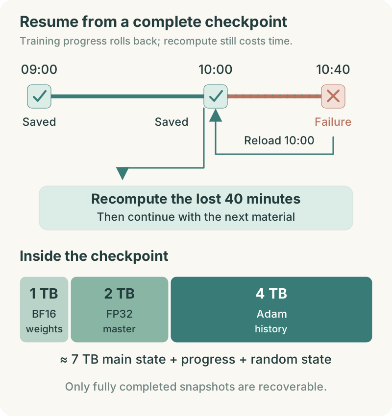
The upper diagram traces the interruption back to the last complete save. The work repeated is the 40 minutes lost after 10 a.m. The lower diagram shows the roughly 7TB of main states in proportion: 1TB of compute weights, 2TB of high-precision master weights, and 4TB of Adam history. Training progress and random states must be saved alongside them.
Training state: All the information needed to continue training, including the model, optimizer, progress, and random states.
Random state: The current position of a random-number generator. Saving it helps recovery continue the same sequence of random operations.
How Do 7TB Spread Across Many GPUs Become One Checkpoint?
The files sit in directories written by many processes. Each GPU holds only the state assigned to it. During a save, it writes those shards and records which part of the model they belong to. Recovery follows those records to return each state to its proper place.
The 80 data-parallel replicas contain duplicate compute weights, but a checkpoint needs only one complete logical model. A distributed saving implementation can have different processes write files together, using many machines without writing all 80 duplicate copies of the weights. We check whether the logical tensors are fully covered, whether any are duplicated, and whether recovery can find their proper destinations.
Megatron provides a distributed checkpointing interface. This plan fixes the implementation and checkpoint format to Core 0.19.2. During acceptance, we compare the inventory produced by an actual save with the expected model state, item by item.
I also checked two different timestamps: when the GPUs resumed computation, and when the background writer actually finished the files. They can differ. Asynchronous saving first creates a consistent snapshot, then lets the background process continue writing. Training can resume once the implementation’s conditions are met. Until all the files are written, the new checkpoint remains in progress.
That snapshot still being written also consumes CPU memory and storage resources. It needs somewhere to live, and background writes compete with data reads. We measure the real snapshot and writing process before choosing concurrency, so “saving in the background” does not become another persistent drag on training.
Shard: One of the pieces into which a large object is divided for storage or processing on different devices.
Consistent snapshot: A set of state copies from the same logical point in time that can restore the system together.
Files Exist. When Can We Call the Save Complete?
Several terabytes in a directory are not enough for me to press Recover. If one machine exits during saving, some shards may be missing. The files already written cannot reconstruct the full training state.
I checked the unique identifier for this save. It starts with an in-progress status. Only after every required shard is written and the metadata and integrity checks pass does it join the completed list. The recovery entry point selects only completed identifiers.
Alongside the framework’s completion callback and checkpoint metadata, we keep an inventory: update time, training step, file counts and sizes, shard coverage, verification results, and archive-copy status. Files requiring additional checks are verified within the storage budget. Completeness should have a record we can inspect.
The system previously pointed to the complete 9 a.m. save. Once the 10 a.m. save was fully ready, it switched the “latest completed” pointer to 10 a.m. in one operation. That is the atomic update here. A reader sees either 9 a.m. or 10 a.m., never a half-complete 10 a.m. Shared-filesystem rename semantics and object-storage commit mechanisms differ, so integration implements and tests this operation for the actual backend.
Looking farther back, the latest three completed saves were still retained according to Part 13’s plan, with room for a fourth being written. Once the new save passes, the retention policy removes the oldest one. Deletion runs separately from completion checks, so a failed save does not erase the existing way back.
Atomic update: A change that appears to its users as one complete operation. Its intermediate state is not read as a finished result.
Integrity check: A check that data is complete and has not changed during transfer or storage.
How Often Should We Save to Waste Less Time?
Recovering the 10 a.m. state made me revisit the hourly save schedule. Saving more often could shorten those lost 40 minutes, but saving itself also takes training time.
I put a three-minute saving pause and an average of one rollback-causing interruption every 24 hours into the table. With hourly saves, the average rollback is about half an hour. Scheduled saving costs 3 ÷ 60, or about 5%. Rollbacks cost 0.5 ÷ 24, or about 2.08%. Detection, restart, and loading time must be added separately.
Saving every two hours reduces the saving share to about 2.5%, while average rollback rises to one hour, or about 4.17%. The sums are close, but recovery time and the failure distribution still affect the choice. We want the frequency that minimizes losses across the whole run.
Setting the interval to 30, 60, 90, and 120 minutes, and initially adding only saving pauses and failure rollbacks, makes the two costs visible:
| Save interval | Saving-pause share | Average rollback share | Combined |
|---|---|---|---|
| 30 minutes | 10.00% | 1.04% | 11.04% |
| 60 minutes | 5.00% | 2.08% | 7.08% |
| 90 minutes | 3.33% | 3.13% | 6.46% |
| 120 minutes | 2.50% | 4.17% | 6.67% |
Save too often, and the pauses take a larger share. Save too rarely, and failures force more repeated computation. With these values, 90 minutes is worth testing alongside the current hourly schedule. The formula below locates the balance more precisely.
The calculation: Why is the balance point about 93 minutes?
Under a simple uniform-failure approximation, let C be the saving-pause duration and M the average interval between interruptions. The two losses associated with a save interval T can be approximated as C ÷ T + T ÷ (2M). This gives a starting point for comparison of T ≈ √(2CM). Substituting three minutes and 24 hours gives roughly 93 minutes. The formula omits correlated failures, changes in recovery time, and conflicts from asynchronous writes. We use it to select hourly and 90-minute comparisons, then decide from actual records.
The three-minute and 24-hour values in this table will be updated from saving-pause and interruption records. The 93-minute balance point will move with them. Part 13’s “fully recoverable within ten minutes” measures the time until the entire save is complete. How long the GPUs are blocked is a separate measurement.
Shorter intervals also put more pressure on storage devices. About 7TB every hour means about 168TB of logical writes per day. Shorten the interval, and that write volume rises. The storage capacity has not changed, but the devices’ workload has.
After a Machine Fails, How Far Should Automatic Restart Go?
Back at the 10:40 a.m. failure, the logs were full of communication timeouts. I preserved the earliest error, confirmed that the job had stopped progressing, and isolated the suspect node. The later timeouts might simply be a chain reaction. The starting point could be an earlier GPU error, network-adapter fault, or process exit.
With the last complete checkpoint located, the next check was whether healthy machines could reconstruct the original cluster size. For now, the on-call operator confirms recovery. Once failure classification, node exclusion, and recovery validation are reliable, common cases can move into an automatic workflow.
As of November 2026, the 0.7.0 release notes for NVIDIA Resiliency Extension include capabilities related to in-job restarts, hot spares, and node health. Automatic recovery is becoming a formal training-system component. This project puts those capabilities through a separate acceptance branch: first check compatibility with Core 0.19.2, the launcher, and the Slurm deployment, then decide whether to integrate them into the main run.
This time, TP8, PP8, and DP80 stay unchanged, and a spare server takes the failed machine’s place. Changing the parallel layout requires revalidating checkpoint resharding, global batch size, optimizer state, and data order. We make that adjustment when there is a clear need.
Recovery can be automated, but it must also know when to stop. If the same material repeatedly triggers an error, the same node keeps failing, or loss persistently deviates after recovery, repeated restarts should stop and investigation should begin. That keeps the cluster from spending the night repeating the same failing stretch.
Hot spare: A prepared spare resource that can take over from a failed resource quickly.
Resharding: Redistributing existing model or optimizer state according to a new division of work among devices.
Recovery Succeeds at the Next Update
Loading finished, and logs began appearing again. I checked the checkpoint identifier, cumulative samples, successful update count, and learning rate, then sampled the identifiers of the next data batch. After a short stretch of updates, I compared the results with the recovery reference from acceptance.
The machines needed checking too. Had every process entered the same stage? Were any shards missing? Had peak GPU memory and throughput returned to similar ranges? If the whole pipeline slowed after replacing one machine, the new node’s software, GPU clocks, network adapters, and cache preparation would be the next places to look.
The shared workspace survived this failure, so recovery used a recent save. A failure that also took out that workspace would send us to the independent archive. It holds complete daily progress and may require a longer rollback, but it still provides a route back. Recovery drills must include both a recent shared save and a retrieval from the archive to establish how long each path takes.
After the next successful update, I recorded the incident: when the last update completed, when the interruption was detected, which save we used, when the next successful update completed, and how many tokens were recomputed. Those records show whether lost time came from slow detection, infrequent saving, or lengthy loading and replacement.
The job interrupted at 10:40 a.m. resumed from its complete 10 a.m. checkpoint. The faulty node was replaced, the data order rejoined, and the repeated 40 minutes remained in the cost ledger. The logs moved forward again. The previous nine days of work were intact.
A roughly 76-day run continues in stretches like this, supported by complete saves and a working recovery path. Once it runs steadily, the next thing worth watching is speed: when every machine looks busy, why might the finish date still keep slipping?
New ideas, straight to your inbox.
AI, engineering, and experiments. One or two useful emails a month.
No spam. Unsubscribe anytime.