[Training a 500B LLM from Scratch] 20/25: The GPUs Look Busy. Why Is Training Still Slow?

I watched the training dashboard for a while. Most of the 5,120 B200s were busy, the logs kept scrolling, and new checkpoints arrived on schedule. Yet when I put completed work beside elapsed time and estimated the finish date again, it landed beyond the original 76 days.

With that question in mind, I opened the logs from a recent stretch of stable operation. Twelve seconds separated two completed parameter updates. In those twelve seconds, the machines read material, computed, exchanged results, and moved the parameters one step forward. To recover time, I had to look inside that interval and find what was holding progress back.

Twelve Seconds in the Log

Part 16 fixed the work in each update: 1,920 sequences of 8K tokens, or 15,728,640 input tokens when the windows are full. Dividing by twelve seconds gives a cluster-wide rate of 1,310,720 input tokens per second.

15,728,640 ÷ 12 = 1,310,720 token/s

Now the speed connected to the schedule: how far through the 10T tokens we had reached, and how long the remainder would take. Following that number back through the records, I checked whether padding was included, whether any updates had been skipped, and whether material replayed after a failure had been counted again as new progress. Comparisons of speed need the same samples, batch size, and scored positions.

Those twelve seconds covered one update during stable training. Saving, evaluation, and recovery consumed additional time, so the finish date had to come from progress across the whole job. This gave us two separate records: update time to locate bottlenecks in the program, and elapsed time to track the schedule.

But the log gave only a total. It did not say which part of the twelve seconds was most worth changing. I captured several consecutive updates and laid their work out on a timeline.

Throughput: Work completed per unit of time. Here, it means non-padding input tokens processed per second across the whole cluster.

Wall-clock time: Time that actually passes, including computation, waiting, and interruptions.

Computation Has Finished, but Something Is Still Running

Nsight Systems lets us view CPU and GPU activity together. I used NVTX to label data loading, forward computation, backward computation, communication, and parameter updates. Capture began after compilation and cache preparation. I first inspected representative processes at the beginning, middle, and end of the pipeline, then compared their corresponding replicas.

Once the timeline opened, a stretch of waiting at the end stood out. On the same scale, computation took eight seconds, followed by four seconds of transfer. The compute track had stopped while the communication track kept extending to the right. The next update had to wait for it.

It was tempting to speed up the network. But communication carries results produced by earlier computation. If a result arrives late, even a faster network must wait. I traced that tail backward to find the last piece of work to hand over its result.

The data input was the easiest place for a controlled comparison. I prepared material of the same shape locally in advance, kept the model and batch unchanged, and ran another short stretch. Updates still took nearly twelve seconds, with no obvious gap at the input. Part 13 had estimated average read demand, and this timeline also gave no reason to blame data supply.

With the material arriving on time, the next question was who finished computing late. The model had eight stages, or PP8. Comparing their sustained durations revealed no stage repeatedly holding up the others. Nor did the 80 data-parallel replicas at the same pipeline position reveal a consistent late arrival.

Zooming in exposed a more specific clue. Some gradients had been ready for a while but had not been sent. They stayed where they were until later computation finished, then transferred together. Part of the wait came from results that were already available and still waiting to leave.

Profiling: Recording when different parts of a program run and how long they take to identify bottlenecks.

NVTX: A tool for adding names and timing markers to program stages so that specific work can be found on a timeline.

PP8: Splitting the model into eight sequential compute stages, which the material passes through in order.

Rank: The identifier of a process in distributed training. Logs use it to distinguish the processes involved in computation and communication.

What should we do when data supply stalls or pipeline stages are uneven?

For a data stall, first locate the earliest point where waiting appears. Repeated reads of small files may call for a different file layout, while preserving samples and boundary rules. Repeated fixed CPU transformations can be done in advance. If the prefetch queue frequently empties, increase its depth gradually while checking memory and cache use. If reads slow down only during checkpoint saves, inspect contention between reads and writes on shared storage. After each change, use the same material to measure waiting again and verify content and order.

For uneven stages, adjust suitable layer assignments first, then measure complete update time, peak GPU memory, and communication. I keep 1,920 sequences per update while addressing implementation issues. More microbatches can spread out pipeline startup and drain overhead, but with other conditions unchanged they also increase the global batch. Learning rate and learning quality then need separate comparisons.

For now, I keep non-interleaved PP8. An interleaved pipeline gives one device several separated stages. It may reduce idle time, while adding scheduling and communication complexity. If the timeline confirms that pipeline bubbles dominate the loss, I will compare supported paths in the Megatron Core 0.19.2 scheduling implementation. Each choice must be evaluated for correctness, memory use, and throughput together.

Send the Results That Are Already Ready

Backward computation produces gradients progressively. Earlier portions can be ready while later portions are still being calculated. When the remaining computation does not depend on the result of that aggregation, both activities can advance together.

Part 15 had already selected overlap for gradient reduction and parameter gathering. Now I needed to understand why that arrangement was not fully visible on the timeline. A blank stretch separated the moment gradients became ready from the moment aggregation began. Following it would reveal the dependency or scheduling choice delaying the send.

I also used nccl-tests to measure communication independently over the same range of message sizes. The network performed normally on its own. The problem lay in how transfers were scheduled during training. That narrowed the change to the aggregation timing of results already available.

After the adjustment, I opened the same section of the timeline again. Computation still took eight seconds. Transfers still represented four seconds of work, but two of them now happened during computation. Only two seconds remained at the end. The next update could begin at the ten-second mark.

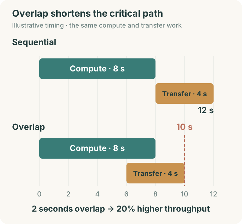
The two transfer bands in the diagram have the same length. Their starting positions changed. All four seconds of transfer remain, with two sharing time with computation. Following the chain of work that the next update must wait for, the whole path is two seconds shorter.

Communication overlap: Performing data transfers while also executing computation that can proceed independently.

Critical path: A chain of dependent work that determines the overall completion time. Shortening it can shorten the complete update.

Further reading: New approaches to communication policies in 2026

The NCCLbpf paper studies adding verifiable policies to NCCL plugins, using information such as message size to adjust communication choices. Its published experiments cover eight B300 GPUs. I treat it as a research direction for programmable communication policies. The official 500B run keeps the validated NCCL combination; new policies need separate comparisons using the actual B200 topology and training messages.

Put Those Ten Seconds Back into Training

The ten-second record came with another obligation. I had changed when gradients were aggregated, so I needed to verify that parameter updates were still correct. I saved the configuration and timeline, then opened update records from before and after the change using identical inputs.

Both runs started from the same parameters, with the same material, batch size, and loss rules. After checking gradients and parameter changes, I also ran each for the same token budget to compare loss and independent validation performance. A change in parallel execution order can introduce numerical differences, so the comparison used an agreed tolerance. Overlapping communication and computation can also keep temporary data in GPU memory at the same time. Peak memory and sustained stability belonged in the check as well.

Only after those checks passed did ten seconds enter the new progress ledger:

15,728,640 ÷ 10 = 1,572,864 token/s

The same material was now processed 20% faster. At last, I could recalculate the finish date that had prompted the investigation.

The Finish Date Moves Forward, but Still Misses the Plan

Part 16 rounded down to complete updates and scheduled 635,782 of them. Saving two seconds each removes 1,271,564 seconds from the computation phase, or about 14.72 days.

At twelve seconds per update, update time alone was about 88.30 days. At ten seconds, it was about 73.59 days. Keeping the 90% calendar availability assumption and adding saving, evaluation, and recovery back into the schedule gives about 98.11 days and 81.76 days respectively. If a measurement window already includes those losses, we convert directly and keep one consistent accounting basis.

The new 81.76-day estimate was much earlier, but the 76-day target was still ahead of us. Earlier planning assumed about 1 PFLOP/s of effective computation per B200. This ten-second record had not yet reached that speed assumption.

Working backward from 76 days made the required pace clear:

76 × 86,400 × 90% ÷ 635,782 ≈ 9.30 seconds per update

From ten seconds to 9.30, about 0.70 seconds remained. That gave the next investigation a specific target. Some communication now overlapped computation. The large block still occupying the timeline was the eight seconds of computation, so that was where I looked next.

How Much of Those Eight Seconds Is Work Done Twice?

Part 15 used recomputation to fit the model in GPU memory. Some intermediate results were discarded and calculated again when needed. That choice saved space, but it also made the same tokens go through additional forward computation.

Putting the memory record beside the compute track revealed room to maneuver. There was memory to spare. Some intermediate results could be kept, avoiding a second calculation later. I listed the repeated work, compared each item's space and time costs, and started with the most worthwhile result to retain. After each change, I ran the same material again to measure the time saved across a complete update and the increase in peak memory. The missing 0.70 seconds gave this tradeoff a clear direction.

By now, the busy GPUs at the beginning made more sense. Repeated computation can keep devices working without letting the model read any new material. The progress I wanted was the same learning task completed sooner.

MFU in the performance report compares useful model work with theoretical hardware capability and helps reveal this distinction. I record it alongside token/s and update time. Increased device activity and faster progress through the material can then be considered separately.

Recomputation: Saving GPU memory by discarding some intermediate results and calculating them again when they are needed later.

MFU: Model FLOPs utilization, the ratio of useful model computation per second to the selected theoretical hardware peak.

How do we calculate MFU and decide whether an operator deserves further optimization?

Using the series' main compute estimate, a 500B dense model needs roughly 6 × 500B operations per token. If the cluster processes S tokens per second, useful model computation is approximately 6 × 500B × S operations per second. Dividing by the theoretical peak of 5,120 GPUs at the selected precision gives an approximate MFU on that basis.

The denominator must specify BF16, FP8, or another precision, and whether it uses a sparse peak. The numerator must state whether additional work such as attention is included. With long contexts, the simple 6N estimate can differ from a full count. Once the basis is fixed, MFU helps compare implementations. Progress through the material and learning results remain separate records.

If the timeline shows a matrix computation repeatedly occupying the critical path, examine its shape, precision, and implementation more closely. A specific computation such as matrix multiplication is called an operator. Operator fusion combines previously separate computations to reduce launch overhead and intermediate reads and writes, while preserving the model's computation rules.

First check how much of the complete update that operator occupies. If it takes two of the ten seconds, reducing it to one second can bring the whole update down to nine only if that saved second lies on the critical path. After the change, check complete update time, peak memory, and learning performance again, rather than recording only the operator's speed.

I archived the validated ten-second configuration beside the before-and-after timelines. Moving some of the transfers earlier brought the estimated finish date from about 98.11 days to 81.76 days. The next experiment had a target in the task record: 9.30 seconds. How much time remained recoverable from computation still needed testing, but now I knew where to begin.

The GPUs were still busy when I returned to the dashboard. This time, there was a traceable explanation for what happened inside that activity and why the finish date had moved forward.

When this main training run ends, I will place a different test in front of the model: read a passage, then answer according to my instructions. Between having read a great deal and becoming a good assistant, there is still some distance to travel.