
[Training a 500B LLM from Scratch] 18/25: When Can the Whole Cluster Begin Training?
Logs scroll across the screen. The program can bring up all 5,120 GPUs. After so much attention to startup, that path finally works, but I have not yet switched it to the main run.
Ahead lies 10T tokens of learning. A small mistake can travel through trillions of them. Is the material read correctly? Are gradients combined correctly? How much speed did the extra machines buy? Scrolling logs still need more specific answers.
I reduce the scale and begin with one update that can be inspected. A small model checks computation; the actual 500B model checks capacity. Then scale rises step by step, ending with saving, failure, and recovery on the whole cluster. Each level earns the next allocation of machine time.
First: Inspect One Update on a Small Dataset
The first acceptance dataset contains only a few dozen examples: long documents, two short documents packed into one window, and padding positions deliberately included to test Part 9's rules.
I choose a model small enough for one GPU, fix its starting weights and material order, and run a complete forward pass, backward pass, and update. Record loss, the number of loss-bearing positions, selected gradients, and updated parameter values. The training process is under examination, so the model stays small enough to inspect each step.
Then split the same material from one large batch into accumulated microbatches. Both paths should agree within a predetermined numerical tolerance. Engineers first check a small, higher-precision control, then establish tolerances at production precision. Precision and operator implementations determine the tolerance; it cannot be relaxed afterward merely to let an error pass.
A subtle mistake hides here when examples have different lengths: simply averaging every microbatch's loss. Without weighting by effective token counts, long and short documents contribute incorrectly. Machines stay busy, loss may even fall, yet the learning objective has shifted.
I check the boundary between the two packed documents again. Keep the second document's tokens and reset position IDs fixed, then replace the first document. Outputs at the second document's valid positions should remain within the same tolerance. This tests the cross-document mask. Padding contributes no loss, while the end marker is learned under the established rule. A few readable examples now provide a correctness reference for trillions of tokens.
Numerical tolerance: The allowed difference when comparing results, accounting for floating-point error.
Control run: A run that holds other conditions fixed while changing the factor being examined, helping identify the source of a difference.
Second: Have Several GPUs Compute the Same Work
Once the single-GPU result agrees, distribute that same small model. Keep material, initial parameters, and global batch unchanged. Enable data, tensor, and pipeline parallelism in turn, checking the result of a complete update.
I separate the checks so a discrepancy has somewhere to be traced. DP checks gradient aggregation for corresponding parameters. TP checks sharded computation and assembly. PP checks forward and backward handoffs and microbatch accumulation. Test each before combining them, narrowing the search if a difference appears.
After the multi-GPU update passes, save and restore with the same configuration. Compare the next sample IDs, learning rate, and update records. Random operations also require their random state to return. Differences between the control and recovery runs must be explainable by the implementation and numerical precision.
The small model's complete results can be compared item by item, establishing a software reference. The memory and communication volume of 500B still require the real model.
Before it enters, test the network separately. NVIDIA's nccl-tests checks both communication correctness and performance. Cover actual message sizes, within-server traffic, and cross-server traffic. Passing one tiny message is followed by large-message and concurrent tests. The data exchanged in training determines the scope.
Third: Find a Starting Scale for the Actual 500B Model
The real 500B model cannot fit its roughly 1TB computation weights on one card. I follow Part 15's grouping to find an initial scale that can accommodate it.
TP8 and PP8 give 64 GPUs per replica, so starting with 64 seems natural. The memory ledger reveals a problem: production shares optimizer state among 80 data-parallel replicas. A single replica must carry more state by itself, increasing its memory burden.
Under Part 15's Core 0.19.2 accounting and equal sharding, each card handles about 7.8125 billion parameters. BF16 weights and FP32 gradients use six bytes; master weights and Adam state use twelve, shared by the DP group. Main state is approximately:
7.8125 billion × (6 + 12 ÷ DP) bytes
At DP1 this is about 140.63GB, at DP8 about 58.59GB, and at DP80 about 48.05GB. Activations, communication buffers, and uneven shards are still outside those figures, so peak usage comes from the actual model.
After comparing the three capacities, I set the first acceptance allocation to 512 GPUs: 64 servers and DP8. It preserves TP8 and PP8 while leaving more activation headroom than DP1. Freeze layer count, width, and stage assignment, then run a few complete updates and record peak memory by stage.
A tight stage sends us back to its input, output, and layer assignment. Compare redistribution and selective recomputation, retaining configuration and throughput for every change. Find a layout that runs continuously before adding replicas.
Peak GPU memory: The highest actual memory use of a GPU during a complete training cycle.
Recomputation: Recalculating intermediate results when backward computation needs them, trading additional computation for less stored state.
Fourth: Check Whether Four Steps of Expansion Are Worthwhile
Once the target model runs continuously, ask how much time more machines buy. I expand through 512, 1,024, 2,560, and 5,120 GPUs, corresponding to DP8, DP16, DP40, and DP80. Each retains TP8, PP8, and the 8K window, creating a consistent comparison.
The global batch remains 1,920 sequences, so accumulated microbatches per group change with replica count:
| Active GPUs | Servers | DP replicas | Microbatches per group |
|---|---|---|---|
| 512 | 64 | 8 | 240 |
| 1,024 | 128 | 16 | 120 |
| 2,560 | 320 | 40 | 48 |
| 5,120 | 640 | 80 | 24 |
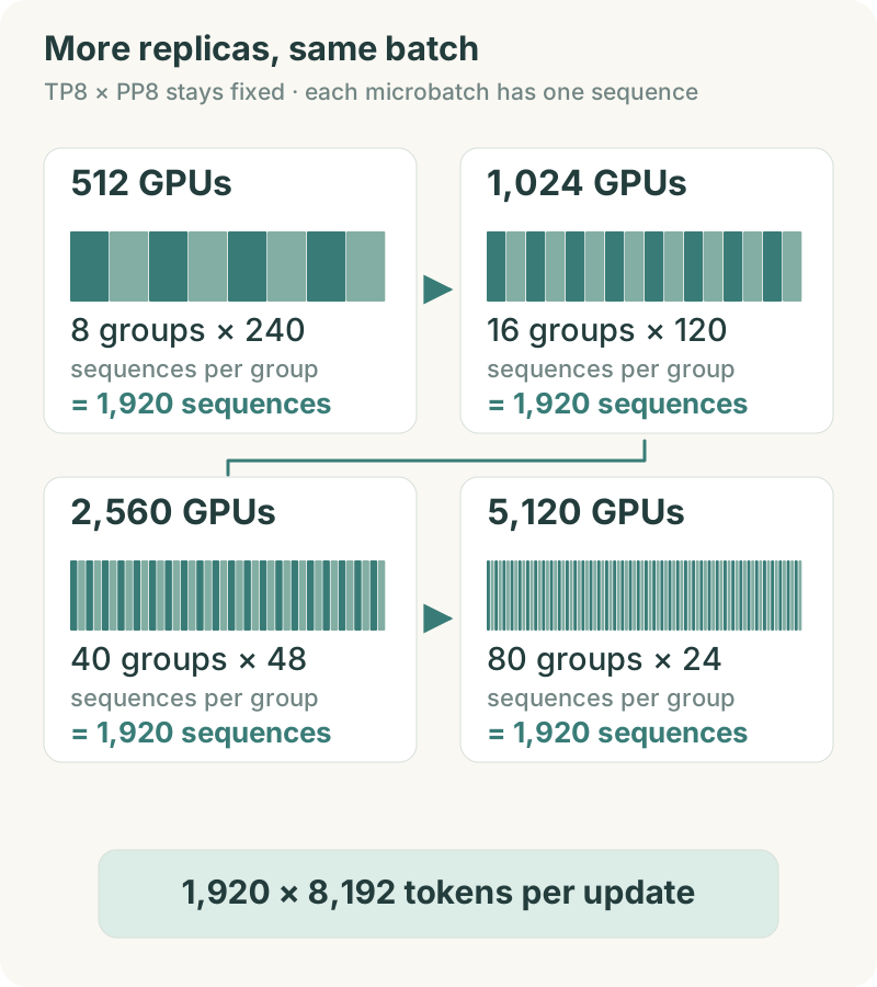
All four scales finish the same work, making speed comparable. More replicas mean fewer microbatches per group, changing the pipeline's fill-and-drain share. More communication participants also lengthen aggregation paths. These are real scaling costs and belong in the results.
Timing needs the same starting line. Complete startup and cache preparation before measuring stable operation. State the window, completed updates, actual non-padding tokens, and whether checkpoints are included. A cold start at one scale cannot be compared directly with steady operation at another.
Enter 180,000 tokens/s at 512 GPUs and 320,000 at 1,024 into the comparison table. The speed ratio is 32÷18, about 1.78. Doubling cards produces 1.78 times the speed, giving this step about 89% scaling efficiency. Apply the same arithmetic to read all four scales together.
The last step deserves particular attention. If moving from 2,560 to 5,120 GPUs brings little speed improvement, stop there and find the bottleneck. Each extra day also consumes facility, electricity, and team time. Locating poor efficiency has value of its own.
Scaling efficiency: Actual speed improvement divided by the ideal proportional improvement as the number of GPUs increases.
Steady measurement window: A period of normal training measured after startup, compilation, and cache preparation have finished.
Fifth: Actually Save, Fail, and Recover
Full-cluster speed needs an escape route. Save Part 13's roughly 7TB checkpoint with the actual model, check its shards, total size, and latest-complete record, then load it again.
Next, deliberately terminate one training process. Follow how others exit, how the scheduler records failure, and whether any process remains occupying a GPU. Quarantine the failed node, substitute a spare, and restore the same progress. This tests code, scheduling, storage, and operations together.
Bring the data team into recovery acceptance too. Sample records must show where the next batch begins, how repeated computation is counted, and whether any material is skipped. Loading parameter files alone cannot establish a correct continuation.
At hardware level, use DCGM diagnostics to inspect GPUs, internal links, power, and temperature-related conditions, then combine them with supplier diagnostics for specific failures. Each tool covers a different area. Retain original errors, nodes, and timestamps so later repair can trace the incident.
After one save and recovery passes, continue across several checkpoint cycles. This plan uses 24 hours as its first observation window for thermal stability, scheduled saves, read variability, and recovery. Repeated failures extend the investigation. Twenty-four hours is a project acceptance choice; the following 76 days still rely on monitoring and recovery throughout operation.
Put Measured Speed Back on the Calendar
With acceptance records collected, I reopen Part 2's calendar. Its 76 days came from planning throughput. The complete target model's speed now takes that place.
At 1.6 million non-padding input tokens per second for the full cluster, 10T requires about 72.34 days of pure computation. At 90% calendar efficiency, it becomes about 80.38 days. Speed and losses change the finish date. Saving, evaluation, recovery, and maintenance records must return to this calendar too.
If throughput already divides by total wall time and includes those losses, use it directly rather than dividing by 90% again. Every tokens-per-second figure needs its time scope so the budget does not discount twice.
I record trial material and GPU time separately as development costs. Configuration comparisons consume an experimental budget; main training accumulates 10T from its chosen starting point. If an accepted trial checkpoint becomes that starting point, explicitly carry forward its consumed material, configuration, and cost.
| Evidence required before the main run | What the owner checks |
|---|---|
| Small-model correctness | Data boundaries, loss normalization, matching gradients and updates |
| Target-model capacity | Peak memory by stage and a stable configuration |
| Four-scale results | Throughput, measurement window, GPU count, and scaling efficiency |
| Save and recovery records | Complete state, material position, spare replacement, and recovery time |
| Updated calendar | Target throughput, operating losses, remaining tokens, and expected completion |
These results allow the configuration to move from experiment into main training. Software version, material version, resource scale, and recovery path all point to records. Scrolling startup logs can now become sustained learning.
There is still a long run ahead. A drill lets us schedule the interruption; a production failure will not wait. Next, we follow an unexpected disconnection and see how to bring progress back.
New ideas, straight to your inbox.
AI, engineering, and experiments. One or two useful emails a month.
No spam. Unsubscribe anytime.