[Training a 500B LLM from Scratch] 15/25: How Do We Split One Model Across 5,120 GPUs?

In the previous article, the small model on our reference machine gained an installation and acceptance path. Replace it with 500B, and capacity is the first obstacle: a single set of computation weights needs 1TB.

I write that next to the B200's 180GB of memory. Five hundred billion parameters at two bytes each far exceed one card. Eight cards provide 1,440GB in total, but their memory remains separate. Software must tell each card what to store, what to compute, and when to pass results to a partner.

And those are only the weights. Gradients, update records, and intermediate results also need space. First divide the model so it fits, then organize the remaining machines to process material faster. I follow one batch through both kinds of work and finally hand the arrangement to the software from the previous article.

One GPU Cannot Hold It. Start by Dividing the Layers

Open Part 4's model diagram. Text becomes numbers and travels through successive layers, each continuing from the preceding result. That order gives us a natural first division.

I split the model into eight sections across eight servers. The first handles the input end, the second continues, and the eighth produces the output. Each section is a stage, retaining its own weights.

The first server computes its layers for a batch and passes the intermediate representation to the second. The moving data describes the processed text. The weights stay with their assigned machine for the next batch.

Reaching the output completes only half the training path. The last stage calculates prediction error, and backward computation returns through the stages, giving each its parameter-update information. Intermediate results travel forward and the corresponding gradients return. The separated layers still form one model: pipeline parallelism, or PP.

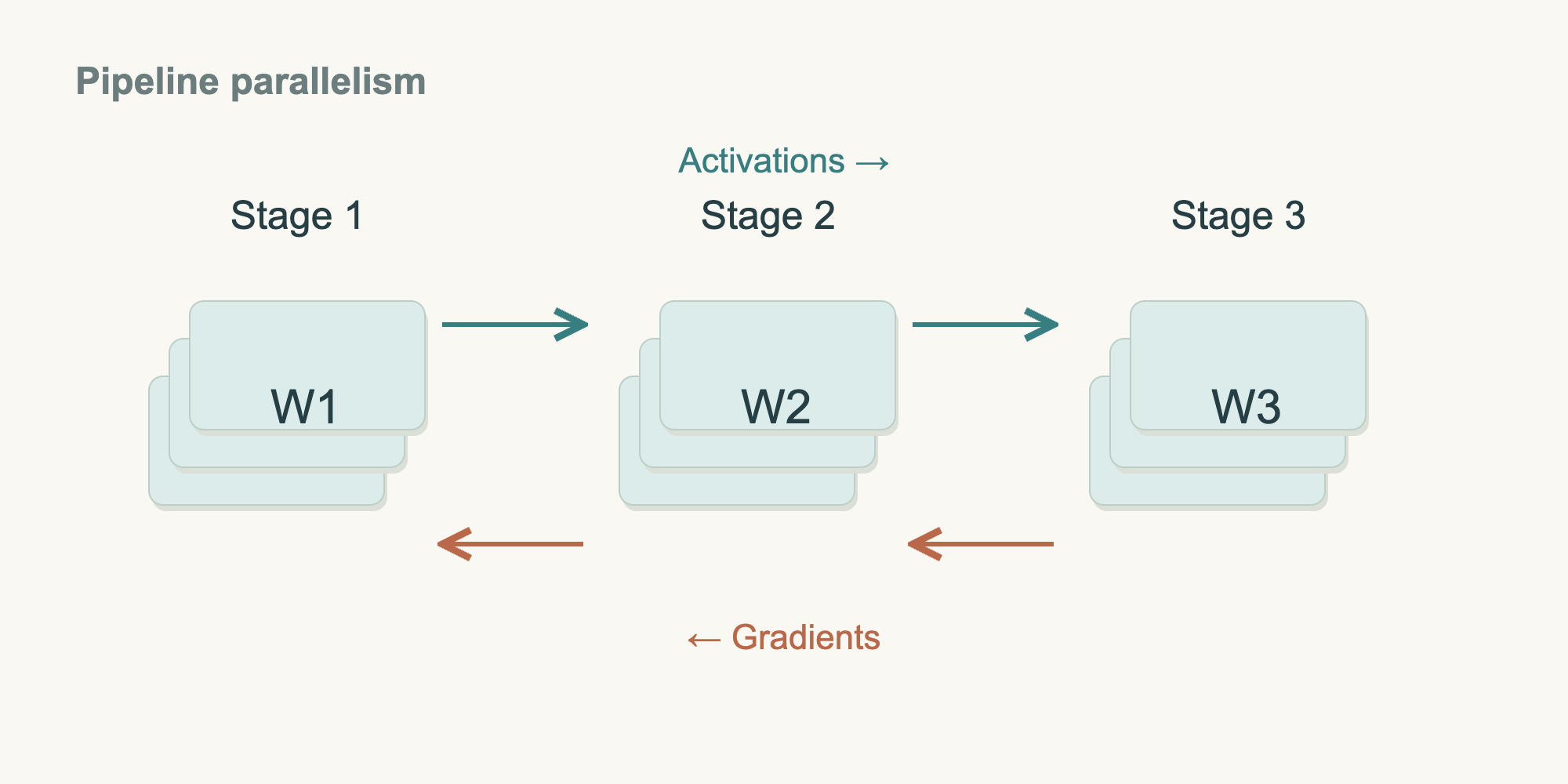
W stays inside each stage. Follow the upper arrows forward with the material, then the lower arrows back with its gradients. Weights remain assigned to their stages; arrows carry this batch's intermediate results and corresponding gradients. The drawing reduces the pipeline to three stages for clarity. The project starts with eight.

Eight needs a reason too. More stages shrink each server's portion but add handoffs and waiting. Start with eight servers, each dividing its work across eight cards, and the main state spreads over 64 GPUs. The memory calculation below will test that choice. Acceptance measures peak memory, stage times, and waiting with continuous microbatches, including the input and output components. Megatron's pipeline implementation schedules those forward passes, backward passes, and transfers.

Eight stages means eight groups of layers. The configuration specifies the boundaries. Similar stage times matter, otherwise one stage stays busy while the next waits.

Pipeline parallelism (PP): Splitting a model into consecutive stages that run on different devices, with each stage passing its results to the next.

Activations: Intermediate results produced as a model processes an input. They pass to later layers, and some must also be kept for backward computation.

Gradient: A value that describes how the error changes when a parameter or intermediate result changes slightly. Training uses gradients to calculate the direction of parameter updates.

Each Server Has a Stage. How Do Its Eight GPUs Cooperate?

The eight stages are assigned, but every server still contains eight GPUs. Divide each layer's large operations among those cards. This within-layer division is tensor parallelism, or TP.

Shrink one layer to two inputs and four outputs. GPU A gets weights producing the first two outputs; GPU B gets those producing the last two. Each receives the required inputs, computes its portion, then exchanges results as subsequent operations require.

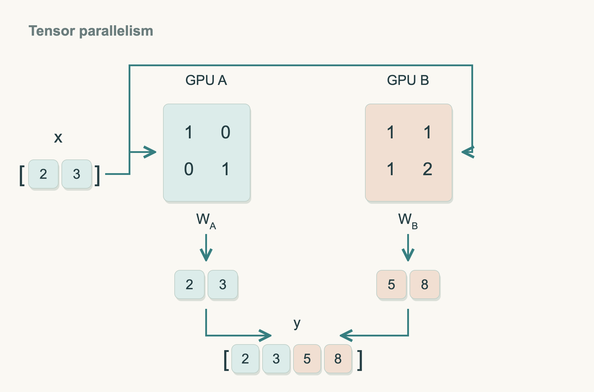
An individual number in the diagram is a scalar; a row forms a vector. With input [2, 3], A uses the left two weight columns to produce [2, 3], and B uses the right two to produce [5, 8]. The final value is 2×1＋3×2＝8. In order, the result remains [2, 3, 5, 8]. Two GPUs illustrate the column split; the real plan uses eight. Some subsequent operations keep shards, while other splits require summation, so communication follows the computation.

The full network uses larger tables of numbers and the same division principle. Megatron supports row- and column-parallel linear layers. Their sequence determines where to exchange or combine results, as the implementation documentation explains. Each GPU retains a portion of the layer's weights and performs its share of computation.

These exchanges recur frequently, making placement important. I keep TP8 inside a server, using NVLink and NVSwitch for frequent within-layer cooperation. Stage handoffs use the cross-server network. This arrangement also follows NVIDIA's parallel deployment guidance.

Together, the two divisions give one complete model a home: eight servers in sequence, eight cards sharing each server's layers, 64 GPUs total. Every batch still passes through every layer. Layer placement and within-layer work simply have separate owners.

Tensor: A set of numbers arranged along one or more dimensions. A matrix is a two-dimensional tensor. Model weights and intermediate results can both be represented as tensors.

Tensor parallelism (TP): Splitting a layer's weights and computation across several GPUs, which exchange results to complete the layer together.

One Group Holds the Model. What Do the Other 79 Do?

I mark off 64 cards beside the total of 5,120. Organizing the rest in the same way gives:

5,120 GPUs ÷ 64 GPUs per group = 80 groups

Each of the 80 groups has one complete copy of the model, internally divided across eight eight-GPU servers. They start from identical parameters and read different material: one group takes one batch, another a different batch, all sampled according to the earlier data recipe.

Different material produces different gradients. Before an update, corresponding contributions are combined: a parameter on the second card of stage three in one group aligns with that same parameter in the other 79 groups. All update from the same combined result. The next round begins with the same model version across groups and new material for each.

This is data parallelism, or DP. It increases how much material one model can process concurrently and still produces one trained model. Megatron's communication groups organize within-layer cooperation, stage handoffs, and corresponding-parameter synchronization separately.

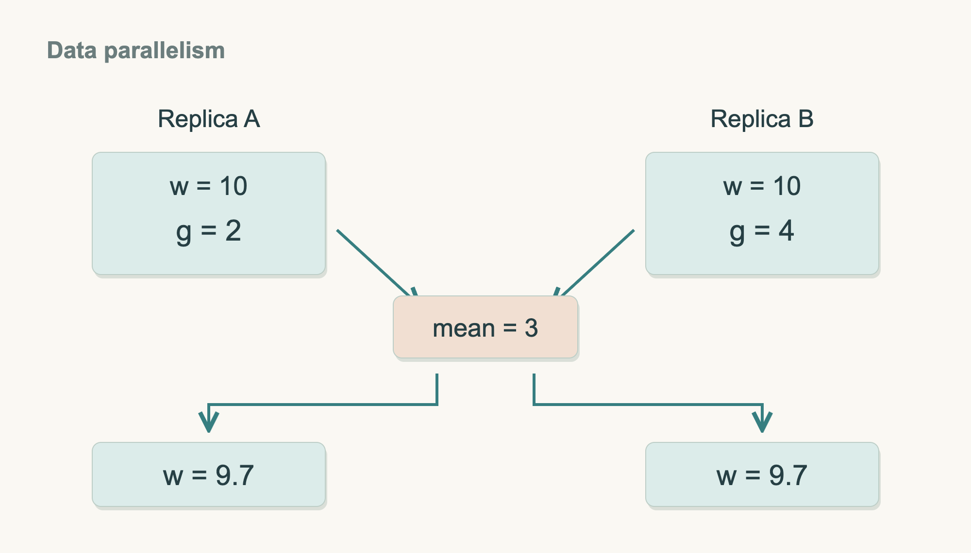
Follow one parameter through the diagram. Both groups begin at 10, process equally weighted microbatches, and obtain gradients 2 and 4. Both use their average, 3. With a learning rate of 0.1 and the simplest SGD rule, both become 10－0.1×3＝9.7. The arithmetic exposes synchronization. The project's Adam also uses historical state to determine its actual step. Each group box represents a complete model carried by 64 GPUs.

This also explains why data parallelism alone could not solve the initial problem. Replicating all 500B parameters on every GPU still exceeds 180GB. First spread one model across 64 GPUs, then replicate the whole group. Capacity and material throughput now have separate solutions.

Put all three levels on one drawing: eight cards in a server, eight servers in a group, and 80 groups. A server box is a machine; a small color block is a GPU's weight shard. Following those levels prevents double-counting devices.

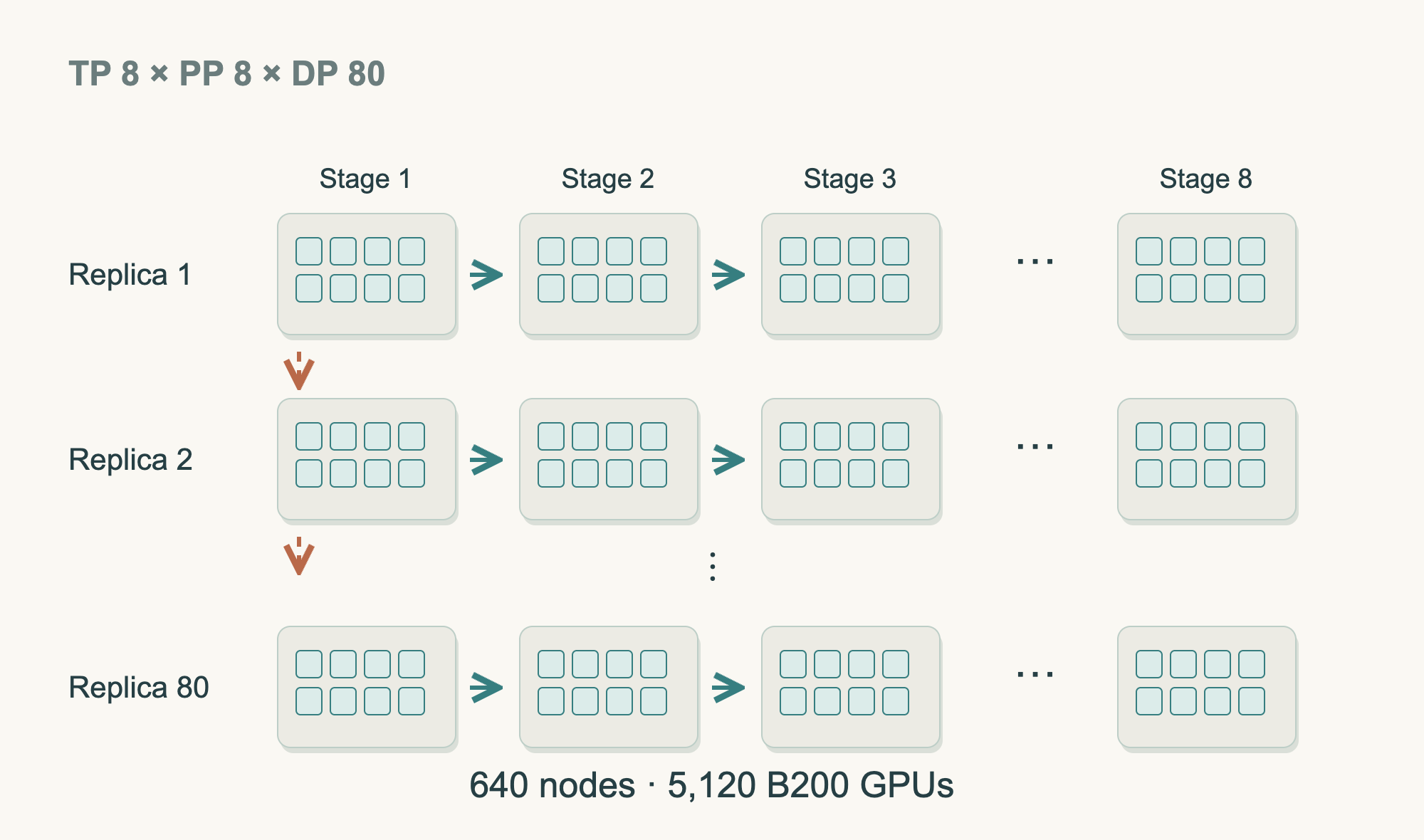
The drawing expands some replicas and one synchronization line. The complete arrangement remains eight servers and 64 GPUs per pipeline, with 80 groups totaling 640 servers and 5,120 GPUs.

Data parallelism (DP): Having multiple computation replicas of the same model read different material, then combining gradients for corresponding parameters to keep their updates consistent.

Model replica: One computational copy of the same model weights. In this article, one replica spans 64 GPUs.

Will the later machines spend all their time waiting?

Capacity is assigned, but gaps remain on the timeline. While the first batch is still in stage one, later stages have nothing to process. Divide an update's material into many microbatches and feed them continuously so the pipeline gradually fills.

As the first microbatch reaches stage two, stage one accepts the second. As it moves farther, other stages work on different microbatches. Training also requires backward computation. Once filled, stages alternate forward and backward work, allowing completed backward passes to release intermediate results.

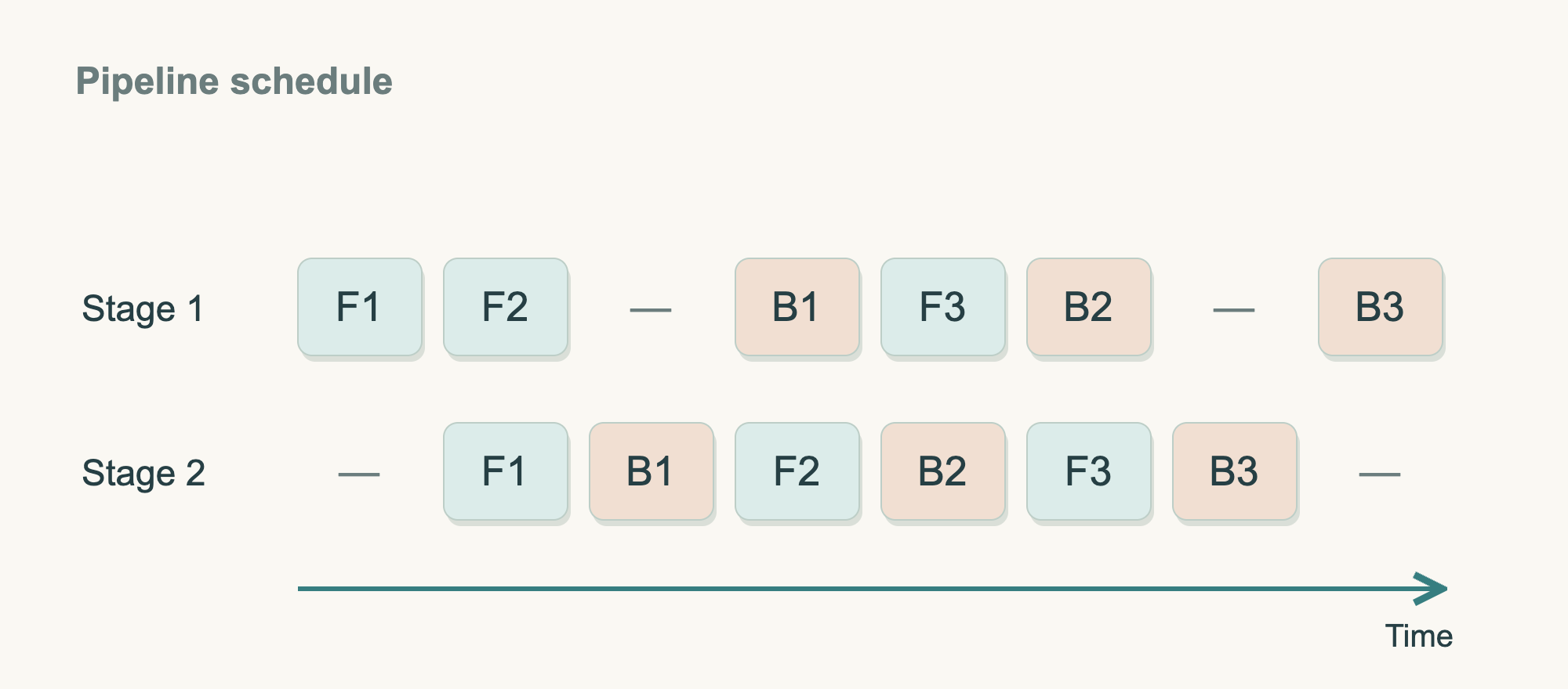
The diagram uses two stages and three microbatches. Follow batch 1: stage one completes F1 before stage two starts it; stage two completes B1 before stage one begins it. Batches 2 and 3 enter as earlier work moves forward. F and B are computation, dashes are waiting, and equal-width cells illustrate order. At the end, no new microbatches enter; remaining backward work drains the pipeline.

Startup and drain still contain bubbles. Too few microbatches leave a large idle share; many microbatches increase the material read before one update. Hardware utilization and learning cadence meet at this choice.

First make the batch arithmetic explicit. Each group accepts one sequence at a time for 32 microbatches, with 80 groups reading different material. One update uses:

1 sequence × 32 small batches × 80 groups = 2,560 training sequences

At 4,096 tokens per sequence, with all positions counted, this is 10,485,760 tokens. Multiply by 80 because those groups read different material. The 64 cards within each group cooperate on the same batch, so do not multiply again. Megatron's microbatch calculator relates global batch, microbatch size, and data-parallel group count in this way.

The values 32 and 4,096 expose the arithmetic. The next article chooses the actual batch and length using memory, bubbles, and learning behavior. Each expansion can then be described precisely: more material per update, or the same material finished sooner.

Microbatch: A small batch of material sent into the pipeline at one time.

Gradient accumulation: Accumulating gradients from several microbatches before performing one parameter update.

Global batch: All training samples used for one parameter update, including samples processed by every data-parallel group.

Pipeline bubble: Idle time when some stages wait for others during pipeline startup, drain, or an imbalance in work.

1F1B: A schedule that alternates one forward pass and one backward pass once the pipeline reaches its steady phase.

Read more: Which pipeline schedule will we use first?

Start with ordinary non-interleaved 1F1B: one consecutive stage per server, using Megatron's existing schedule. Interleaving introduces multiple virtual stages and changes bubbles and communication. Measure the ordinary setup first, then compare that additional arrangement with the same model and batch.

The Computation Fits, but the Update Ledger Is Still Large

After dividing the model, another large item remains on the memory list: the records used for updates. Weight computation has been assigned; the ledger can also be divided.

Each parameter usually has a high-precision master copy and optimizer histories. Eighty groups update the same parameter set, making 80 copies of these records expensive.

Open one parameter's ledger: a computation copy, a precise master copy, and two Adam histories tracking gradient direction and scale. Part 16 examines the update itself. Here, choose who keeps the ledger. All 80 corresponding members need one parameter; one member can perform its update and share the new computation value.

I enable Megatron's distributed optimizer to assign these records among corresponding DP members. Each GPU receives combined gradients for its portion, updates that portion using its ledger, and shares the new computation weights. Computation copies remain complete while update records are distributed. The 0.19.2 documentation describes this flow.

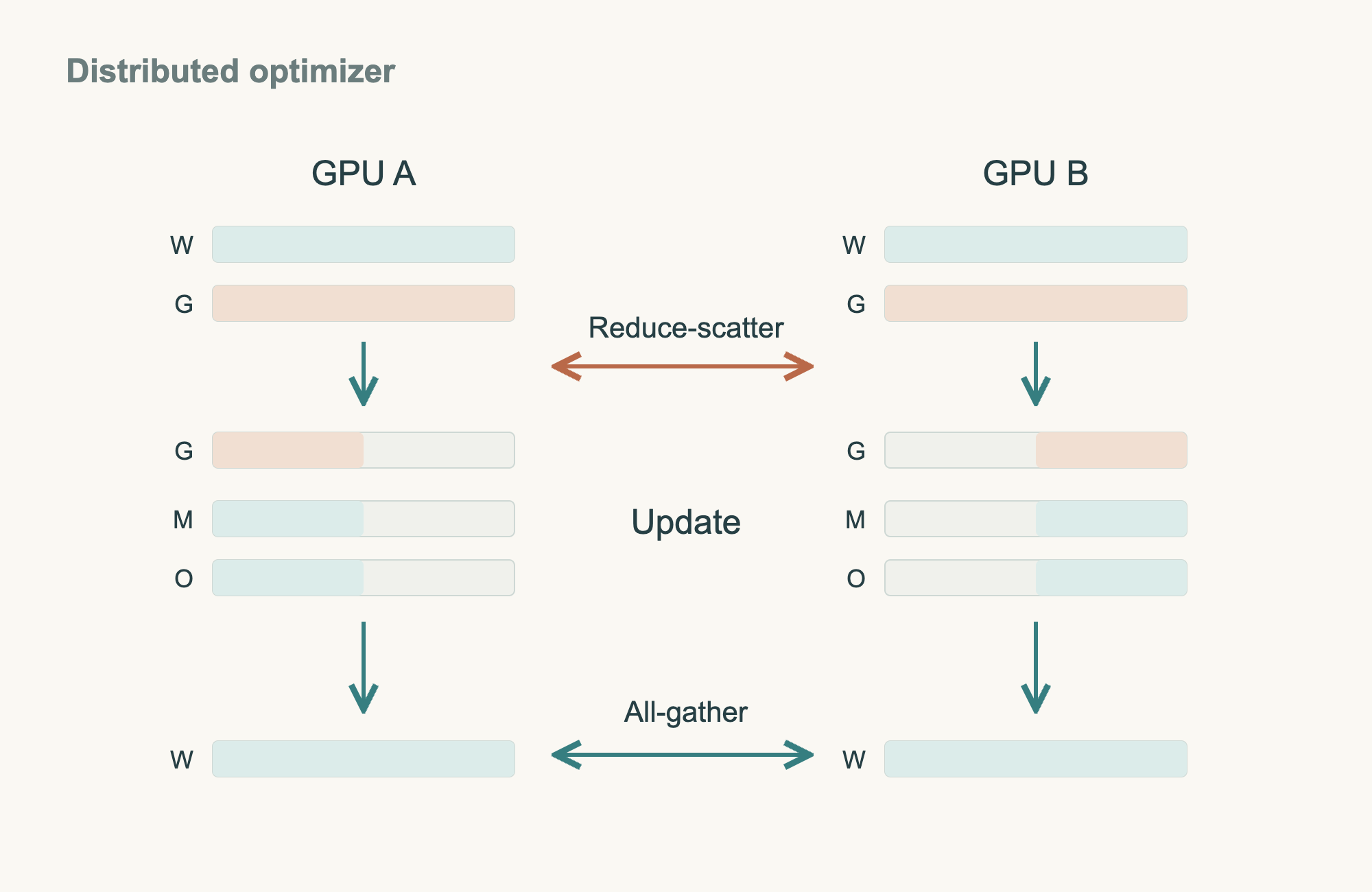
W is computation weights, G gradients, M master weights, and O Adam history. Bars represent state blocks; half-bars are further shards. During computation, two DP members both have the corresponding BF16 weights and FP32 gradient buffers. At update time, gradients are combined and each member receives its assigned portion, updates with local M and O, then exchanges new W. The next computation again uses matching weights while the larger ledgers remain split. The drawing uses two members; the project shares them among 80 corresponding members.

Reduce-scatter: Combining data at corresponding positions, then giving different portions of the combined result to different members. Here, it sends combined gradients to the member responsible for updating those parameters.

All-gather: Collecting the different portions held by members so that each member receives the complete data it needs. Here, it collects the updated computation weights.

How can the 2026 implementation reduce waiting further?

With destinations established, look for waiting on the timeline. Transfer a gradient block as soon as it is ready while continuing computation that does not depend on that transfer. Update only after all required contributions arrive. Previously idle time can now carry useful work.

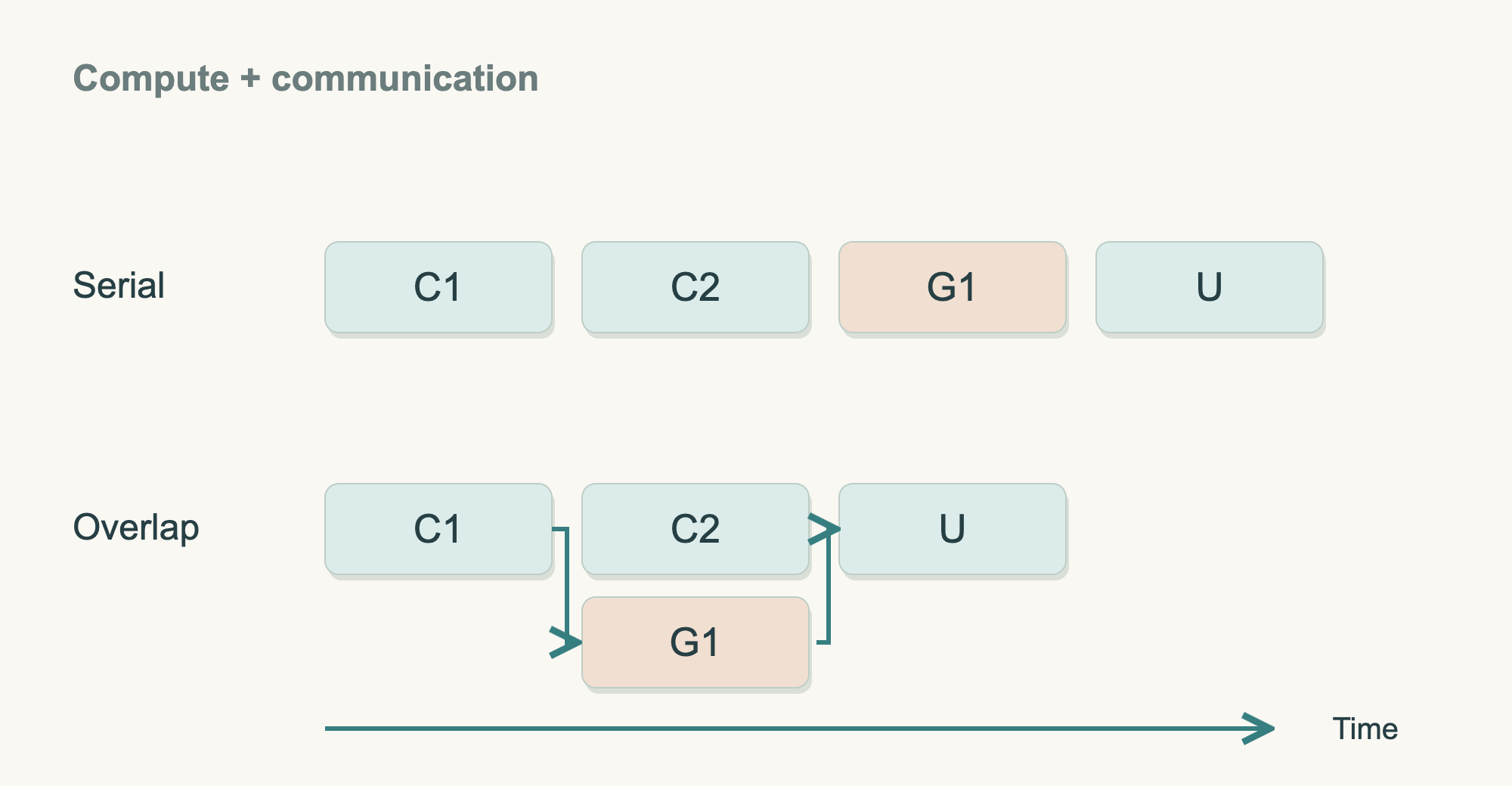
C1 and C2 are computation blocks, G1 transfers the gradients from C1, and U updates. The upper timeline performs them sequentially; the lower overlaps C2 with G1. Dependencies remain: G1 follows C1, and U waits for required results. Equal cells explain this relationship; the actual overlap comes from the measured training timeline.

Overlap has developed over many years. Our implementation is Megatron Core 0.19.2, released in September 2026. Its pinned configuration offers gradient-reduction and parameter-gather overlap, both off by default. Our target enables both with the distributed optimizer. The same version's validation supports this with ordinary non-interleaved pipelines. First verify results with overlap off, then enable each option and compare peak memory, step time, and waiting.

Communication and computation overlap: Transferring data that is ready while performing computation that does not depend on that transfer.

The software choice refines memory accounting. Earlier planning used 16 bytes per parameter. BF16 computation weights, FP32 accumulated gradients, and Adam state now require 18 before sharding. Higher-precision gradient accumulation adds two bytes, refining 500B main state from 8TB to 9TB. Distributing the ledger reduces per-card pressure again.

Read more: How does one GPU's main state fall from about 141 GB to about 48 GB?

We use decimal GB and start with an ideal equal split of parameters across TP8 and PP8. Each GPU handles 500B ÷ 64, or about 7.8125B parameters. The real model's input and output layers, small amounts of replicated parameters, and differences in stage workloads still need separate checks.

State	Bytes per parameter	Placement in our plan
BF16 computation weights	2	Each data-parallel replica keeps its corresponding shard
FP32 accumulated gradients	4	This implementation retains the main gradient buffer
FP32 master weights	4	Shared across 80 corresponding data-parallel members
Two FP32 Adam states	8	Shared across 80 corresponding data-parallel members

Without sharding, the total is 18 bytes per parameter: 7.8125B × 18, or about 140.625 GB.

With the distributed optimizer, the documented theoretical accounting is 6 + 12 ÷ DP bytes per parameter. Substituting DP80 gives:

7.8125B × (6 + 12 ÷ 80) = 48.046875 GB

This includes the main state in the table. Acceptance testing must also measure the peaks caused by activations, communication buffers, temporary workspaces, memory alignment, and differences between stages. We therefore cannot simply subtract 48 GB from the B200's nominal 180 GB and treat the remainder as guaranteed usable capacity.

Part 13's 7 TB checkpoint estimate still applies. It stores 2 bytes of computation weights, 4 bytes of master weights, and 8 bytes of Adam state, for 14 bytes per parameter. This archive, written after a parameter update, does not store gradients. Sharding changes which machine saves each portion; it does not multiply the model's 7 TB of logical state by 80.

FSDP can reduce resident weights further, splitting weights, gradients, and optimizer state across DP members and gathering weights when computation needs them. We first validate TP, PP, and the distributed optimizer, keeping frequent within-layer work inside an eight-GPU server on our chosen Megatron path. FSDP remains a comparison for memory and cross-server communication under the same workload; PyTorch's explanation follows its gathering process.

Read more: How does FSDP split the storage of weights too?

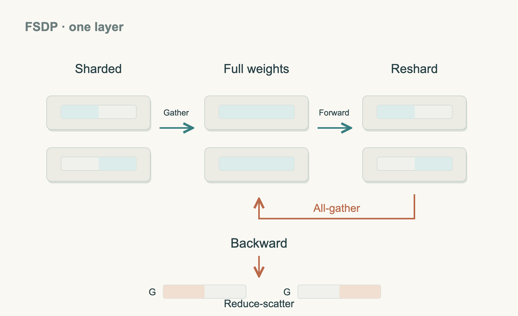
Follow one layer through the diagram. Teal bars represent weights, terracotta bars represent gradients, and a colored half-bar is the shard held by that member. Normally, each member holds only its assigned weights, gradients, and update records. When it is time to compute this layer, the members first gather the weights it needs. With resharding after computation, the temporary full weights are released after this layer's forward pass and gathered again when the backward pass needs them. The resulting gradients are combined and delivered as shards to their respective updaters. This reduces memory that must remain occupied, while adding communication to gather weights. It is an alternative for comparison; our plan still starts with the combination selected above.

Implementations continued to develop this approach in 2026. The Megatron Core 0.19.0 release notes from August 2026 list improvements to FSDP forward weight-gather overlap and hybrid sharding. The current version's HFSDP documentation further divides members into inner and outer groups. Weights and gradients are sharded within an inner group, while the larger optimizer records are sharded across all members.

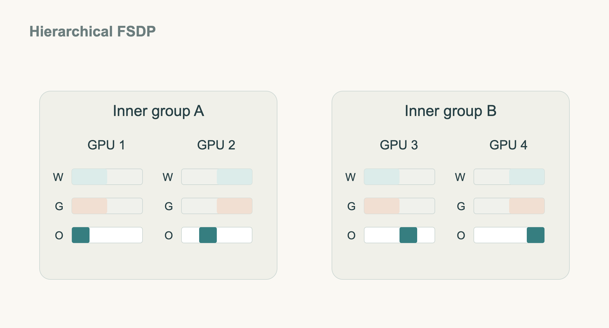
Look at the two groups. Each can assemble the same complete W and G, but each of its two members holds only half. O represents optimizer records, with each of the four members holding one quarter. This confines frequent weight gathering to a smaller inner group. It is another grouping worth measuring when memory is limited. Our current plan already uses the eight GPUs in a server for TP. A comparison with HFSDP would require rearranging the groups and checking whether communication happens within a server or between servers.

Optimizer state: Historical records that an optimizer uses to decide how to update a parameter. Adam keeps two such states for each parameter.

Distributed optimizer: An implementation that shards the master weights and optimizer records needed for parameter updates, while coordinating gradient reduction, updates, and weight synchronization.

Put Every Division Back on One GPU Count

Return to the original 1TB-versus-180GB comparison. The assignment now fits one line: eight cards share layers inside each server, eight servers form a pipeline, 80 pipelines process different material, and update records are distributed.

TP 8 × PP 8 × DP 80 = 5,120 GPUs

Enable Megatron sequence parallelism within those same groups to reduce duplicated activations for some operations without multiplying devices again. Start at CP1 with no additional context division. Validate the three main arrangements first; longer sequences can motivate another split and a recalculated DP count.

Read more: Where do sequence, context, and expert parallelism fit?

Sequence parallelism splits activations for some operations along the sequence dimension and is commonly paired with TP. It uses the same existing GPU group as tensor parallelism. Megatron's parallelism guide lists the relevant settings.

Context parallelism, or CP, distributes the processing of one long sequence across more devices. Attention still obtains the context it needs through communication. This can reduce activation memory per GPU while adding new communication arrangements. The official CP documentation explains the mechanism and support requirements. We start with CP1 as our acceptance baseline. If we use CP2 for a later long-sequence phase while keeping TP8 and PP8, the same 5,120 GPUs give us DP40.

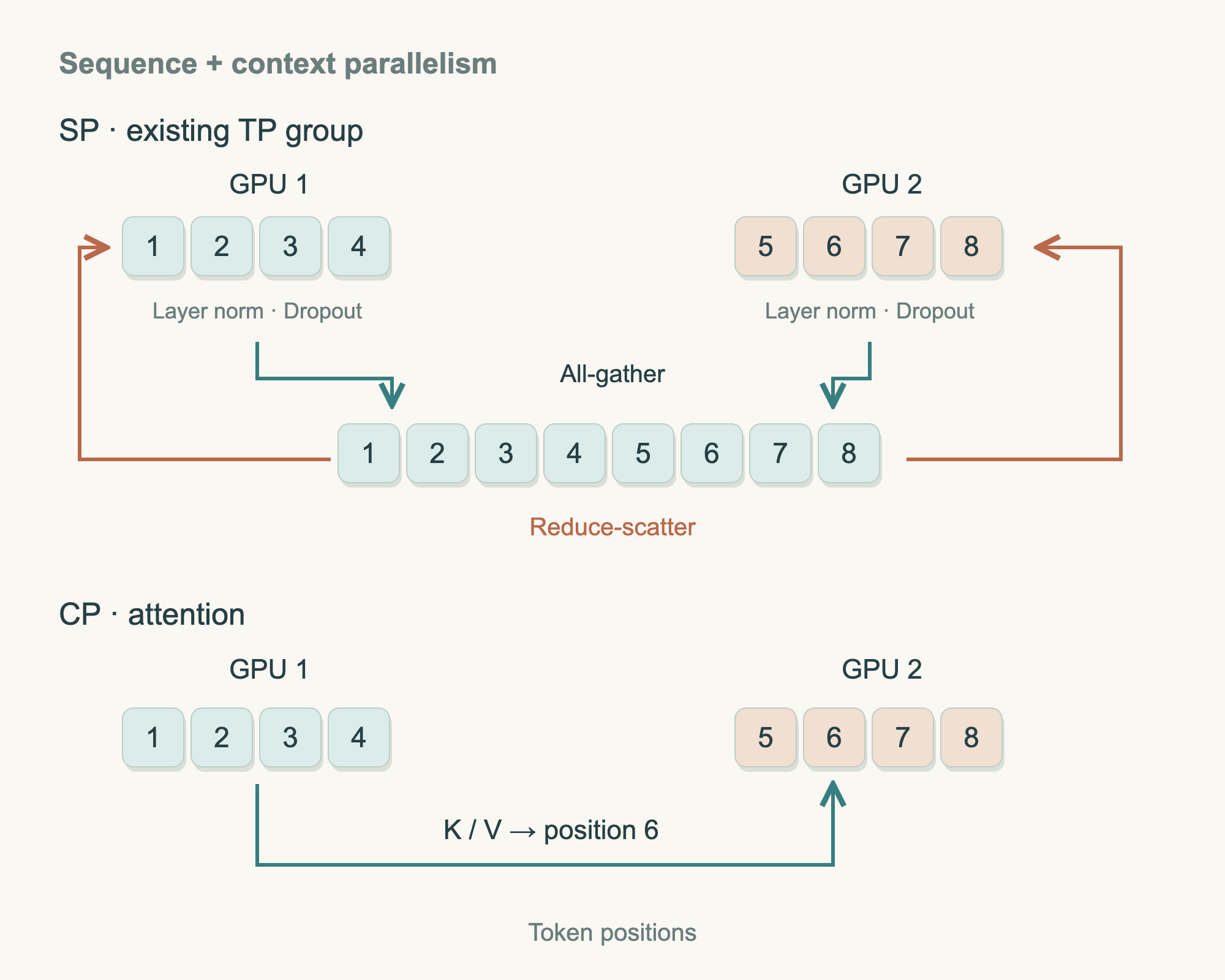
The numbers 1 through 8 mark token positions, not values inside a vector. Behind each cell is a full set of activations for that position, which forms a vector. Each GPU member shown is one GPU, not an entire server.

Start with the upper half. Positions 1 through 8 of the same sequence are divided between two members of the existing TP group. Each stores and processes the activations for some operations, such as layer norm and dropout. All-gather collects the shards where the full sequence activations are needed. Reduce-scatter combines results and shards the corresponding output again. These communications follow the needs of the surrounding computations and backpropagation. This is sequence parallelism, with no additional group of devices.

The lower half adds a new context-parallel dimension for processing the long sequence. Two members handle different positions. During attention, they still exchange the context information they need to connect relationships across the entire sequence. The diagram shows position 6 reading K/V from earlier positions. The associated gradients must also travel between members during training's backward pass. Contiguous positions are used here for clarity; actual implementations also arrange position assignments to balance the workload.

Layer norm means layer normalization, which adjusts the scale of a set of numbers. Dropout randomly masks some values in training configurations that use it. K and V are the attention keys and values discussed in Part 6. The current token uses them to obtain the context it is allowed to read.

Long material can also vary in length from one batch to another. Dynamic-CP, described by NVIDIA in January 2026, chooses the context-parallel size according to each microbatch's actual length and workload. Short material uses fewer devices, and long material uses more. It is designed for workloads with variable-length material.

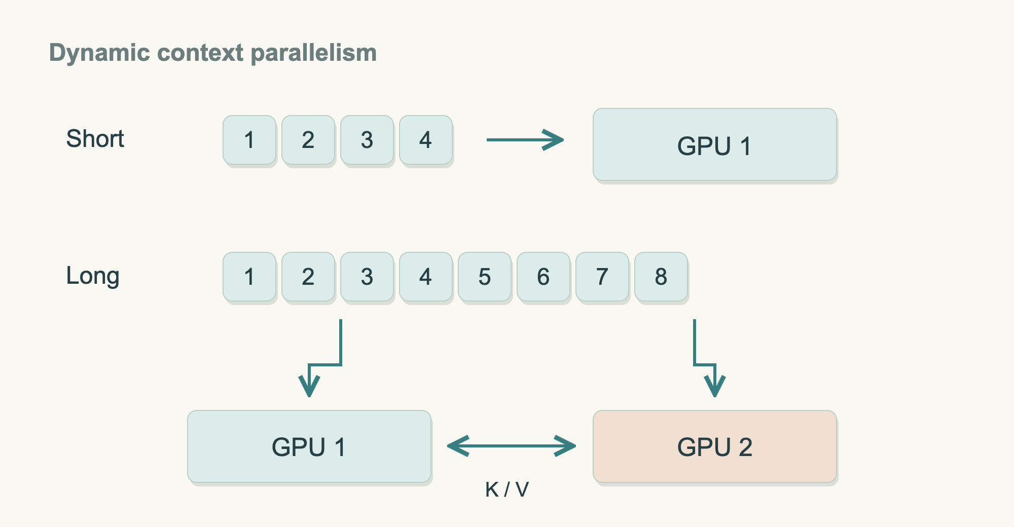
The diagram gives the short material to one member and splits the long material between two. The long material still uses communication to obtain the context required by attention. Four cells and eight cells illustrate the difference in length; actual switching depends on workload and configuration. We will first establish a CP1 baseline with a fixed sequence length. In a later long-context or variable-length phase, we will compare static CP and Dynamic-CP using the same number of effective tokens. Training loss will also be aggregated according to the tokens that actually contribute to learning, so short and long batches contribute in proportion to their effective data volume.

Expert parallelism applies to the MoE models discussed in Part 5, placing different experts on different devices. This series currently plans procurement and training for a 500B dense model, so our configuration uses the division of work for a dense model.

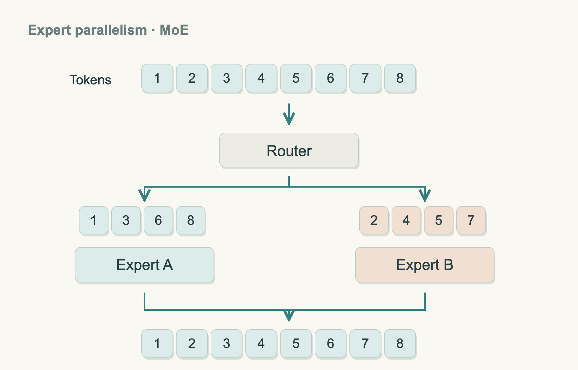
The numbers 1 through 8 represent token positions, each with a vector behind it. Each expert on a GPU holds a set of neural-network parameters. A router selects experts for each token and sends the corresponding vectors to the devices that host them. After the experts compute their outputs, the results return, are combined using the routing weights, and are restored to the original token order. Here, the experts are distributed across devices, and different tokens can choose different experts. The diagram shows only one expert path per token for clarity. An actual configuration can choose multiple experts for one token. This applies to MoE models. Our planned 500B dense model uses the TP, PP, and DP combination described earlier.

Recomputation can also reduce the intermediate results saved for long sequences. We retain the necessary inputs and recalculate some activations during the backward pass. This adds computation. We will first measure peak memory at the selected sequence length, then compare the cost of selective recomputation. The official activation recomputation documentation describes the implementation.

Sequence parallelism: Splitting the storage and processing of activations for some operations along token positions within an existing tensor-parallel group.

How does the software from the previous article carry out this plan?

The drawing still needs to become a running job. I return to the Part 14 environment, request 640 eight-GPU servers, and specify the image plus TP8, PP8, and CP1. The program derives DP80 from 5,120 GPU processes.

Slurm allocates machines, and the node launchers start one training process per GPU, 5,120 in total. Pyxis uses Enroot to bring them into the chosen container. Every machine receives the same software and configuration, with GPU access provided by the installed driver and runtime.

After allocation, Megatron divides the model, creates communication groups, and schedules computation. The second card in stage three has same-server partners sharing its layers, preceding and following stages, and matching cards in the other 79 replicas. The pinned grouping implementation establishes these relationships separately; scheduling then orders each microbatch's forward pass, backward pass, and update.

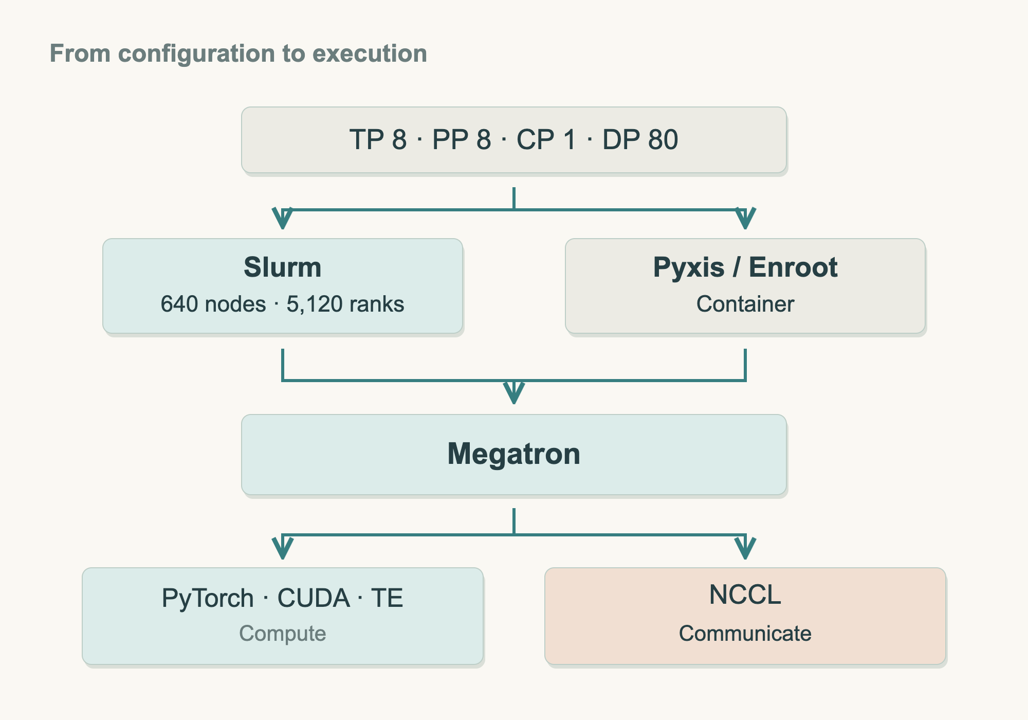
Follow the diagram downward. Resource requests become processes, and Megatron assigns model and material. PyTorch performs tensor operations and automatic differentiation; CUDA and implementations such as Transformer Engine execute on GPUs. Exchanges pass through PyTorch's distributed interfaces and communication paths such as NCCL. NVLink and NVSwitch carry within-server traffic; InfiniBand carries cross-server traffic. Both paths are accepted before production training.

The software names now correspond to concrete work: Megatron chooses when and with whom to communicate; NCCL performs the exchange. Slurm manages resources and jobs, while Pyxis and Enroot provide the environment. After parameters update, Part 13's checkpoint path saves progress, completing the chain.

Validate first with a small model, comparing computation and updates before and after division within agreed tolerances. Then place the target model on the planned groups and inspect peak memory, time, waiting, and communication by stage. Heavy input or output components call for new stage boundaries. Excessive waiting calls for comparing divisions under the same model, batch, and length. Every adjustment answers an observed problem.

Add the 80 groups gradually, recording actual token throughput, material per update, and recovery after restart throughout expansion. These measurements ultimately calibrate Part 2's estimated schedule.

The model that did not fit one card now has an assigned machine for every part and three kinds of partners for each card. How much material to use per update, and how far to move the parameters, remain open. Next, we put batch size, sequence length, and update cadence into one configuration and decide how these 5,120 GPUs will learn.