
[Training a 500B LLM from Scratch] 16/25: How Much Do We Read, and How Do We Update the Model?
The parallel layout is drawn: 5,120 GPUs form 80 groups, each using 64 cards to compute one 500B model. Back in the training configuration, several fields remain empty before startup: how much context to read, how much material to collect before updating, and how far to change the parameters.
The machines' division of labor is clear. These numbers must now connect it to the model's step-by-step learning.
I follow one piece of material: the window it enters, the group that receives it, the feedback it produces, and how that feedback becomes an update. Along this path, the 10T plan can reach each individual learning step.
First, decide how far the model can connect the context
Here is a 6,000-token tutorial. It defines a data structure near the beginning and gives the complete usage near the end. A 4,096-token window cuts it apart, leaving the later section unable to see the definition. At 8,192, the whole tutorial can enter together and preserve that relationship.
I set the initial main-training length to 8,192 tokens. It gives ordinary long documents and code passages more continuous context while keeping the first memory and computation tests at the 8K scale. Here, 8K means 8,192 tokens. Chinese characters and English words must pass through the tokenizer selected in Part 9 before conversion.
Connecting the context increases computation. Ordinary causal attention permits L×(L+1)÷2 position relationships in a sequence of length L. At 4,096, that is about 8.39 million; at 8,192, about 33.56 million, roughly four times per sequence. Holding total tokens fixed halves the number of 8K sequences relative to 4K, but still approximately doubles these relationships overall. This concerns attention; the model has substantial other work, so total training time requires measurement.
Short documents enter the window under the rules in Part 9: independent documents attend to their own preceding content, position numbers restart at document boundaries, and the end-of-document marker is learned. Cross-document predictions and padding positions do not contribute to the loss. Related files from the same project first become one training unit. Packing two unrelated short documents into an 8K sequence does not automatically turn them into one long document.
Seeing that cost, I keep initial acceptance within the same boundary: establish that 8K runs with TP8, PP8, CP1, and sequence parallelism, then evaluate which tasks improve with longer windows. A later long-context stage takes its share from the cumulative 10T, with the compute budget recalculated.
Sequence length: The number of token positions received by one model computation. Each main-training sequence here has 8,192 input positions.
Loss: A value that measures the gap between the model's predictions and the training targets. Training uses it to calculate how the parameters should change.
Each group reads one sequence, then accumulates several results
The tutorial enters its 8K window and the model carried by 64 GPUs. A forward pass predicts; backward computation follows the error and leaves gradients. A gradient describes how a small parameter change near its current value affects loss. I initially give each group one sequence per microbatch, setting microbatch size to 1.
One sequence leaves room for intermediate results. Part 15 counted main-state memory, but material creates additional state as it passes through the model. Raising the microbatch from 1 to 2 places two sequences together and usually increases this pressure. Once the 500B layer count, width, and stage boundaries are fixed, each stage's peak still needs measurement. Starting at one makes that added cost easier to see.
After one sequence, gradients exist but parameters stay in place. Read the next sequence and accumulate feedback for 24 microbatches. All 80 groups do the same, combine their contributions, then perform one update:
1 sequence per microbatch per group × 24 microbatches per group × 80 groups = 1,920 sequences per update
1,920 sequences × 8,192 input tokens per sequence = 15,728,640 input tokens per update
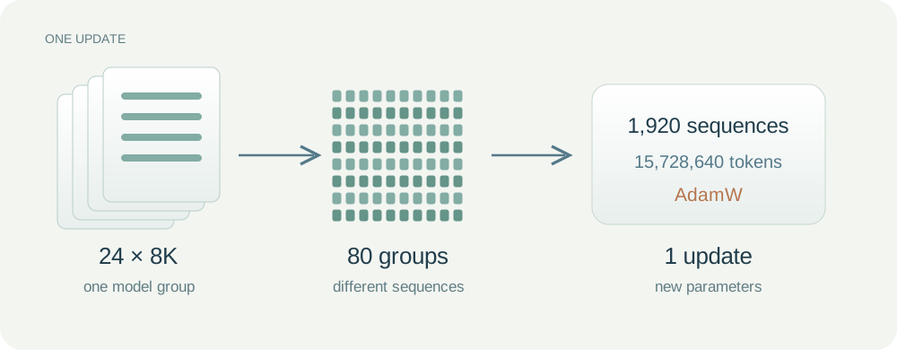
Each thin sheet in the figure represents an 8K sequence. Follow one group reading 24 sequences on the left, then the 80 groups combining their contributions in the middle, and finally one update on the right. The 64 GPUs within each group cooperate on the same material, which is why we multiply by 80 here. The next batch uses the new parameters after the update finishes.
The calculator gives 15,728,640 tokens for filled input windows. Part 9 excludes some boundary predictions from loss, leaving slightly fewer learning targets. Logs separately count input tokens, loss-bearing tokens, and padding. The cumulative 10T follows the earlier material-reading definition; padding is not material, and rereading material counts again.
Microbatch size: The number of sequences one model replica receives in a small pipeline batch. Here it is 1.
Gradient accumulation: Processing several microbatches and accumulating their gradients before making one parameter update.
Global batch size: The total number of sequences used for one parameter update. Here it is 1,920. Multiplying by sequence length gives the token count.
Why start near 16M rather than 8M or 32M?
After entering 24, I compare it with 12 and 48. This number changes both the feedback collected per update and how continuously the eight-stage pipeline can work.
A concrete reference is Meta's published Llama 3 405B training plan. It used 4M, 8M, and 16M-token batches, increasing with progress, and 8K as a main-training length. Its scale is close enough to 500B to help choose initial comparison points. Learning effects still need comparison on our data and model.
With 80 groups, one sequence per microbatch, and 8K per sequence, all three choices divide evenly:
| Input tokens per update | Global sequence count | Microbatches per group | Ideal pipeline idle fraction |
|---|---|---|---|
| 7,864,320, about 8M | 960 | 12 | About 36.8% |
| 15,728,640, about 16M | 1,920 | 24 | About 22.6% |
| 31,457,280, about 32M | 3,840 | 48 | About 12.7% |
Calculating this table introduces 8 minus 1, or 7: the number of handoffs between eight stages. Imagine just two stages first: when the first starts, the second waits for the first microbatch to arrive. After the last microbatch enters, downstream work still needs time to finish. Here, one time unit combines a stage’s forward and backward computation for one microbatch. With eight evenly balanced stages, the ideal model counts the combined fill-and-drain overhead as seven of these time units. Processing 24 microbatches therefore takes approximately 24 useful units plus seven overhead units. The idle fraction is 7 ÷ 31, or about 22.6%.
The last column considers only the fill and drain of an ordinary non-interleaved pipeline. Assuming equal computation across eight stages and ignoring communication and other waiting, the idle fraction is approximately (8 − 1) ÷ (microbatches + 8 − 1). This explains the direction of change as we add microbatches. Actual utilization comes from the execution timeline.
The 8M setting updates more often, but each update has only 12 microbatches, so filling and draining take a larger share. The 32M setting can keep the pipeline busy more easily, but it makes only half as many parameter updates as 16M after reading the same total amount. Validation tells us whether the extra material in each batch delivers the corresponding benefit.
After weighing both ends, I retain the middle 15.73M setting first. It lowers ideal idle share from roughly 37% to 23%, while preserving twice the update opportunities of 32M. Compare 8M and 32M against it at equal tokens for validation loss and at equal validation performance for elapsed time. If 8M learns the same amount from less material, lower hardware efficiency may pay off. If 32M learns similarly with better throughput, there is evidence to enlarge the batch.
The August 2026 OpenEuroLLM study studies learning rate and batch size together and distinguishes training stages. It reminds us to revisit the learning rate when changing the batch. Here, we first use a fixed batch configuration to establish a reproducible comparison, then decide whether to increase the batch as training progresses.
Pipeline bubble: Time when some stages temporarily have no computation to perform because of pipeline startup, drain or waiting.
Validation loss: Prediction error measured on held-out material that does not update the parameters, used to track learning.
After reading, what actually changes the parameters?
The 80 groups' gradients are together, and the batch's feedback is complete. They indicate directions in which parameters can move to reduce prediction error. That feedback must now change the stored parameters; otherwise the next batch still uses the old model.
The optimizer handles this step. It receives parameters and gradients and applies a rule to produce new parameters. Some rules use only the current gradient; others retain previous changes. Choosing the rule determines how each batch's feedback becomes learning.
I pick one parameter and work through the simplest gradient-descent update. Its old value is 0.5 and this batch's gradient is +0.2. Locally, the positive sign says increasing it raises loss. Moving toward lower loss therefore means reducing it slightly.
Use 0.01 as the learning rate for this calculation:
New parameter = old parameter − learning rate × gradient = 0.5 − 0.01 × 0.2 = 0.498
If the gradient were −0.2, the same rule would increase the parameter to 0.502. The gradient describes local change; the learning rate controls how far we move along that direction. An overly large step can pass a useful location, while a very small step may produce little improvement. After an update, we process the next batch, calculate the loss and gradients again, and repeat.
The parameters in a 500B model are an enormous collection of these numbers. Together, they determine how attention, feed-forward networks and other components compute. The optimizer updates them in tensor batches, gradually changing how the whole model predicts.
Gradient: The local sensitivity of the loss to changes in parameters. Each component describes the direction and rate of loss change for a small change in the corresponding parameter.
Backpropagation: Starting from the loss and working backward through the model's computation to calculate parameter gradients.
Optimizer: An algorithm that updates model parameters using gradients and other information under a chosen rule.
Learning rate: A coefficient that controls the overall size of a parameter update.
Why remember earlier gradients?
Follow that rule across batches and another problem appears. Different material makes gradients fluctuate: the parameter moves down, then the next batch pushes it up. Listening only to the current batch can make updates swing back and forth.
I want a repeated direction to persist, with an occasional opposing signal changing only part of it. A weighted average of recent gradients provides that behavior. This use of historical direction is momentum: consider several rounds of feedback together before choosing the next direction.
Steadier direction leaves another difference. Gradient scales vary by parameter. One often sits near 0.1, another near 10. Multiplying by the same learning rate makes the latter move much more. Each parameter's own history should help set its update scale.
Adam combines these ideas. It keeps two records per parameter: a weighted average of recent gradients to help form the update direction, and a weighted average of squared gradients whose square root supplies a scale. The update divides the former by the latter, then multiplies by the learning rate. Parameters with persistently large gradients have a larger scale denominator, while those with smaller gradients are adjusted against their own scale.
Adam can therefore produce a different update value for each parameter, while we still set a learning rate for training as a whole. The historical records adjust relative update scales across parameters, and the learning rate controls the overall step size. Both work together in one update.
Momentum: A method that accumulates recent gradient directions so parameter updates also reflect earlier feedback.
Adam: An optimizer that uses histories of gradients and squared gradients to adjust each parameter's update direction and scale.
From Adam to AdamW: what do we choose?
The parameters themselves also need attention to magnitude. A small continuing pull toward zero can constrain selected weights while they fit the material. This is weight decay.
AdamW handles that shrinkage separately from Adam's gradient-based update. Gradient history determines how to reduce prediction loss, while a separate coefficient controls weight decay. We can configure these two effects separately and inspect the resulting update rule more clearly.
At this point, I enter AdamW in the first configuration. It adjusts updates from each parameter's gradient history, our Megatron toolchain has a distributed implementation, and the preceding memory and checkpoint plans already reserve space for its states. Continuing with it lets updates, state sharding, and recovery be validated together.
With the algorithm selected, return to the learning rate controlling overall step size. The initial peak is 0.00008, or 8×10⁻⁵, using the earlier 405B plan's peak as the scale for a central 500B trial value. The previous 0.01 illustrated basic gradient descent; 0.00008 is the peak candidate for this project.
Check another update on one parameter. After Adam's history, scale adjustment, and initial correction, its update value is 0.5. At the peak rate, the gradient-based update term is 0.00008×0.5=0.00004. Every parameter has its own history and therefore its own update value.
The division also includes ε = 10⁻⁸ to avoid an excessively small denominator. We start with a weight-decay coefficient of 0.1. Multiplied by the current learning rate, it determines how much to shrink on this update. At the peak learning rate, the decay term alone gives a multiplier of 1 − 0.00008 × 0.1 = 0.999992. Continuing with a parameter of 0.5, shrinkage gives 0.499996; subtracting Adam's 0.00004 then gives 0.499956. Both effects are now visible in one update. PyTorch's AdamW algorithm description lists this order. Biases, normalization parameters and other groups follow explicit grouping rules, and startup logs must record which groups receive decay.
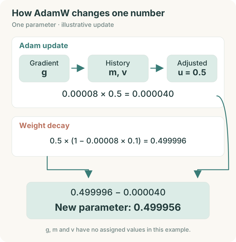
The figure follows one parameter, so every value is a single number. Here, g is the current gradient, m and v are the two historical records, and u is the update value after history and scale adjustment. The example assigns u = 0.5; it does not assign values to g, m or v. Follow the two paths downward: one calculates the 0.00004 to subtract, the other shrinks the old parameter of 0.5 to 0.499996. They combine into a new parameter of 0.499956.
How long do the histories remember, and how do we configure them?
We also give the two historical records explicit starting settings. The first uses β₁ = 0.9 and the second β₂ = 0.95. Each retains 90% or 95% of its previous record, respectively, then adds the new contribution from the current gradient or its square. Using roughly 1 ÷ (1 − β) to interpret memory length, these correspond to scales of about 10 and 20 updates. Adam also corrects the initially small records at the start of training. We choose these values so recent changes can register within a few dozen updates, then observe the gradients and validation curves.
These options correspond to Core 0.19.2's optimizer configuration. Here, β₂ = 0.95 and weight decay of 0.1 are deliberate experimental choices for this plan, preserved in the configuration file.
A batch can also produce unusually large feedback. I set gradient clipping to 1.0. A whole-model norm of 2 halves the gradients without changing direction; a norm of 0.5 leaves them unchanged. The norm must be combined correctly over the model's relevant shards, rather than clipping each card independently to 1. Logs retain the pre-clipping norm and clipping frequency to reveal overly aggressive rates or unusual material.
AdamW: An optimizer that uses gradient history to adjust parameter updates and applies weight decay separately.
Weight decay: Gradually shrinking selected weights toward zero during training to constrain their magnitude.
Gradient norm: A value that combines many gradient components to measure their overall size.
Gradient clipping: Scaling down an excessively large gradient while preserving its direction, limiting the input magnitude to an update.
The learning rate needs a beginning and an ending
The peak is set, but it should not be applied unchanged from the first step to the last. Parameters and their histories are new, so I allow a warmup: rise linearly from 0 to 0.00008, then gradually decrease.
Initially reserve about 20B input tokens, 0.2% of 10T, for warmup. Rounded upward to 1,272 full updates, that is 20,006,830,080 input tokens. Roughly 1,300 startup updates give us a starting interval, judged by loss, gradients, and parameter changes near the peak. Continued deterioration there calls for comparing 40B warmup or a lower peak from the same initial state. A warmup percentage alone cannot establish stability.
After warmup, cosine decay lowers the rate to 0.000008 by the end of the budget, one tenth of the peak. Updates continue, but the gradually smaller steps help refine the directions learned earlier. We choose cosine decay because this run has an explicit cumulative training budget, so its start, peak and endpoint form a complete curve.
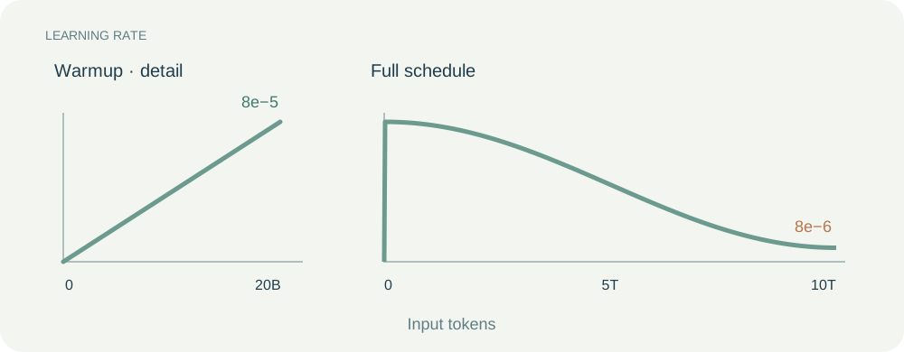
The horizontal axis is cumulative input tokens and the vertical axis is learning rate. The left side enlarges warmup; the right shows the full training schedule. This is a planned schedule, not a measured loss curve. Halfway through the remaining progress after warmup, the learning rate sits midway between its peak and final value, at about 0.000044.
The pinned scheduler implementation supports linear warmup and cosine decay. To locate progress by material read even when batches change, we configure the schedule in samples. One sample has 8,192 input tokens, so 20.00683B corresponds to 2,442,240 samples. Logs convert this back to tokens so the displayed progress matches our material accounting.
Warmup: A startup period that raises the learning rate from a smaller value to its target peak.
Learning-rate schedule: A rule that determines how the learning rate changes as training progresses.
How do these choices reach the software we installed?
One update is complete on paper; now hand it to Part 14's software. Slurm, containers, and Megatron have their places, and Part 15's parallel layout is configured. Slurm allocates machines, torchrun starts GPU processes, and those processes run the Megatron-LM entry point. It reads our arguments and creates the model and optimizer. After each batch's gradients are combined, the loop updates parameters and advances the learning-rate schedule.
Along this path, AdamW and the learning rate belong in Megatron's arguments. Slurm continues to organize machines and jobs. Keeping those duties clear identifies the configuration to change when changing learning behavior.
Two similar names make me check twice. AdamW decides how parameters change from gradients and history; --use-distributed-optimizer decides how those histories are stored and updated across GPUs. One is the algorithm, the other Part 15's distributed implementation. Enable both to preserve AdamW's rule while sharing state among 80 data-parallel replicas.
In Core 0.19.2, the launch argument is --optimizer adam. That version's construction code reads decoupled_weight_decay, which is enabled by default, and passes it to Transformer Engine's FusedAdam. When this switch is true, it executes AdamW. Transformer Engine 2.18's implementation states the same relationship. “Fused” means that update computations are combined to reduce GPU launch overhead.
After checking the implementation, write the choice explicitly: use the adam entry, retain this version's enabled decoupled decay, set the coefficient to 0.1, and enable the distributed optimizer. The interface determines spelling; these settings together determine the update rule.
Distributed optimizer: An implementation that distributes optimizer states and related update work across devices. It can support a specific update algorithm such as AdamW.
Put the choices into one configuration
Walk through again and every number has a place. Each model group reads 24 sequences of 8K; 80 groups form a global batch of 1,920. Aggregate and clip gradients, update through AdamW at the current learning rate, then use the new parameters for the next batch. Main state retains Part 15's BF16 computation weights, FP32 accumulated gradients, and distributed optimizer.
| Setting | First planned value | What it determines |
|---|---|---|
| Model and training material | 500B dense model, about 10T cumulative input tokens | Scale and total work |
| Parallel layout | TP8, PP8, DP80, CP1, with sequence parallelism | How 5,120 GPUs cooperate |
| Sequence length | 8,192 | Reading window for one sequence |
| Microbatch / global batch | 1 / 1,920 sequences | Each group accumulates 24 microbatches per update |
| Optimizer | AdamW, β₁ 0.9, β₂ 0.95, ε 10⁻⁸ | How gradient history is used |
| Weight decay / gradient clipping | 0.1 / global norm 1.0 | Constraints on weight and gradient magnitude |
| Learning rate | Warm up from 0 to 8 × 10⁻⁵, then cosine decay to 8 × 10⁻⁶ | Overall update size |
| Warmup amount | 2,442,240 sequences, or 1,272 updates | Startup over about 20B input tokens |
| Precision and state | BF16 compute weights, FP32 gradients and Adam state | Memory accounting from Part 15 |
The full run also needs the model architecture, tokenizer, data paths and document-boundary handling selected earlier. Layer count and hidden width determine the actual 500B model and each stage's memory use. Once the architecture is frozen, we save these file versions alongside the table.
Expand: How do we express this with Core 0.19.2 arguments?
Part 14 uses the Megatron-LM training entry point and container recipe from the Core 0.19.2 tag. The following argument fragment goes to that entry point alongside the existing model, data and runtime arguments. It describes this article's training choices. Slurm resource requests and torchrun rendezvous settings remain in the launch script. Argument names have been checked against that version's argument definitions.
--tensor-model-parallel-size 8
--pipeline-model-parallel-size 8
--context-parallel-size 1
--sequence-parallel
--micro-batch-size 1
--global-batch-size 1920
--seq-length 8192
--bf16
--use-distributed-optimizer
--overlap-grad-reduce
--overlap-param-gather
--optimizer adam
--adam-beta1 0.9
--adam-beta2 0.95
--adam-eps 1e-8
--weight-decay 0.1
--weight-decay-incr-style constant
--clip-grad 1.0
--lr 8e-5
--min-lr 8e-6
--lr-warmup-init 0
--lr-decay-style cosine
--lr-warmup-samples 2442240
--train-samples 1220701440
--lr-decay-samples 1220701440
Read these arguments in four groups:
| What we tell the program | Corresponding settings |
|---|---|
| Which update rule to use and how to retain history | --optimizer adam, --adam-beta1 0.9, --adam-beta2 0.95, --adam-eps 1e-8 |
| How to constrain weights and oversized gradients | --weight-decay 0.1, --weight-decay-incr-style constant, --clip-grad 1.0 |
| How the learning rate starts, changes and ends | --lr 8e-5, --min-lr 8e-6, --lr-warmup-init 0, --lr-decay-style cosine, plus the two samples arguments for warmup and decay length |
| How states are shared and communication overlaps | --use-distributed-optimizer, --overlap-grad-reduce, --overlap-param-gather |
We explicitly set the weight-decay schedule to constant: its coefficient stays at 0.1, while the actual shrinkage on each update still follows the learning rate. Warmup length is --lr-warmup-samples 2442240; the decay endpoint is --lr-decay-samples 1220701440. These samples are sequences. Multiplying by 8,192 input tokens per sequence gives the material quantities in the article.
Decoupled weight decay retains its true default in this pinned version's OptimizerConfig, and we check it when constructing the optimizer. If we later call Core directly through a Python entry point, we also set that field to true. BF16 mode retains FP32 gradient accumulation, without enabling the extra option that converts main gradients to BF16. Document boundaries, positions and loss rules remain separate checks in the data path, as specified in Part 9.
10T is not exactly divisible by 15,728,640. We initially take 635,782 complete updates: 1,220,701,440 samples and 9,999,986,196,480 input tokens. This is 13,803,520 short of 10T, or about 0.000138%. The executable baseline rounds down to a complete update and records the difference in the budget. An exact 10T requirement would need separate handling of the final batch size and masks; one additional full update would slightly exceed the budget.
The same version's training loop advances the learning-rate schedule only after a successful parameter update. A skipped update may still increase the consumed-sample counter. The update counts and endpoints above therefore assume that all updates succeed. Runtime records separate reading progress, successful updates and skipped updates; recovery restores optimizer and scheduler state together.
After startup, how do we confirm the settings took effect?
Saving a configuration still leaves execution to check. In the first small-model acceptance run, I require the parsed optimizer configuration, actual type, and parameter groups. They must show AdamW mode, β₁=0.9, β₂=0.95, ε=10⁻⁸, and which groups use decay 0.1 or 0.
Core's default grouping skips decay for biases and one-dimensional parameters. We check that list against the actual model and save it. During training, we record the current learning rate, gradient norm before clipping, whether clipping occurred, and whether the update succeeded, connecting each configuration choice to a real action.
For example, the learning rate should rise along the planned warmup schedule and approach 0.00008 near the peak. For a sampled parameter that receives decay, we can recalculate the next step from its old value, gradient and two historical records, confirming both the Adam update and separate weight decay. Once this small check passes, we proceed to validation of the full training configuration.
Before the main run, how do we show this configuration is worth using?
First verify one update. Use a small model on a few machines and fix the material. Compare direct global-batch processing with accumulated microbatches, checking loss normalization, gradients, and parameter changes. Inspect boundaries too: learn the end marker, mask cross-document prediction, exclude padding from training volume. Later curves will then have a consistent meaning.
Once updates agree, place the frozen 500B architecture in the planned groups. Measure several full updates, then extend the trial to observe steady throughput. Record each stage's peak memory, forward/backward time, communication waits, and non-padding input tokens per second. Microbatch size is already 1. If activations remain too large, compare selective recomputation and inspect stage boundaries. Every adjustment requires new 8K throughput measurements and a revised duration estimate.
Once the machines run continuously, ask how well the configuration learns. Screen obviously unsuitable ranges on smaller models, then test promising settings at target scale. Compare batches near 8M, 16M, and 32M, with limited peak-rate trials around 4×10⁻⁵, 8×10⁻⁵, and 1.2×10⁻⁴. Keep data order, token budget, and validation set fixed. Short runs establish numerical and system behavior; trials covering warmup and some peak-rate training then compare validation loss. Small-model screening saves cost, while target-scale evidence makes the final choice.
These comparisons are development experiments with separately recorded consumption. Only the selected main run continues toward the main-training 10T. When a loss spike appears, examine the material, gradients and update record together. If the same content repeatedly triggers the problem, inspect the data. If many ordinary batches deteriorate after increasing the learning rate, lower the peak or extend warmup, then repeat from the same checkpoint.
Finish by deliberately saving, stopping, and restoring. Check the next batch, learning rate, optimizer records, and cumulative counters. Part 13's checkpoint arrangement now connects to this exact training progress.
The empty fields are finally filled: 8K windows, one sequence at a time per group, 24 accumulated microbatches, and an update after combining 80 groups. AdamW follows a rising then falling learning rate as material approaches 10T. Changes in the logs can now be traced to specific settings.
I save the file. Next, how do 640 servers receive that same configuration and start together in one job?
New ideas, straight to your inbox.
AI, engineering, and experiments. One or two useful emails a month.
No spam. Unsubscribe anytime.